


Overview
Welcome to the world of OSPF (Open Shortest Path First) routing. This protocol was developed to replace RIP and it is a classless Link State routing protocol that uses areas so as to scale better. This chapter is divided into four parts since it is too broad. The concepts we will learn will be useful in not only the ICND 1, ICND 2 and CCNA composite exam but also in the real world.
In part 1 of this chapter, we will review concepts on link-state routing protocols and learn how they work. We will then look at the OSPF packets and discuss the algorithm that OSPF uses to find the best part. We will then configure OSPF in a single area and finally we will learn some of the commands that can be used to verify OSPF.
The concepts you will learn in this part, will be important in understanding OSPF in the routing world and will be useful as you progress in your studies in CCNP and CCIE.
Link-state routing protocols
As we learnt in a previous chapter, internal routing protocols fall into two categories, distance vector routing protocols and link state routing protocols. OSPF falls in the link-state routing protocol category. We also used an analogy of a tourist trying to find his destination using a map and said that this is how link state routing protocols work.
Link-state protocols work by calculating the cost along the path from a source network to the destination network and use the SPF algorithm which was developed by Edsger Dijkstra. the steps shown below describe how Link-state routing protocols such as OSPF work.
- All the routers that have been configured with the link-state routing protocol in a domain will learn about the directly connected networks.
- The routers that share a link will recognize the neighboring routers and form relationships.
- When this relationship has been formed, they will share their directly connected routes with each other. This is done when the router in a link-state routing protocol sends a packet that contains the routes.
- The neighbors that receive this information will then propagate it to other neighbors.
- When all the neighbors know oof all the routes, each router will use the information to create a “MAP” to all the destinations in the networks.
- When this map has been created, the SPF (Shortest Path First) algorithm, is run to determine which the best route to a particular remote network is.
This is the basic operation of Link state routing protocols such as OSPF and IS-IS, we will continue learning these steps in more detail as we continue in the world of OSPF.
OSPF operation
In OSPF, the process above is followed, however, the terms differ and are discussed in this section. There are key concepts that we need to know, so as to understand the operation of OSPF.
OSPF packets types
There are 5 different types of packets in OSPF that we need to understand. These are:
- Hello – this are the first messages that are sent by routers that have been configured with OSPF. they use the multicast IP address specially reserved for OSPF which is 224.0.0.5. the hello packets are used sent so as to discover neighbors and maintain relationships – adjacency with them.
NOTE: hello packets are multicast at 10 second intervals in multicast and point to point networks and 30 seconds on NBMA networks. We will explore more of this at a later stage.
in OSPF, the hello packets have three main tasks as listed below.
- Discovery and establishment of neighbor adjacencies
- Advertisesment on OSPF parameters needed to form neighbor relationship
- Election of the DR (Designated Router) and the BDR (Backup Designated Router) in multi-access networks.
- DBD (Database Description) – this packet is a list which contains a summary of routes that have been learnt by a particular router in the routing domain. The router that receives this packet, checks the list against its own link-state database, to discover any missing routes.
- LSR – Link-state request – when a router discovers that it is missing some routes as a result of the information contained in a DBD packet it has received, it sends this packet to the router that informed it of the missing routes, requesting more detailed information on the missing routes. This is done so that it can update its link-state database with these missing routes.
- LSU – Link-State Update – this packet is sent by a router that has information on any missing routes. It contains detailed information about a particular route, including the next-hop information and the cost to reach the particular route that was requested using an LSR.
- LSAck – Link-State Acknowledgment – this is a packet that is sent to confirm that a router has received an LSU.
NOTE: at this stage, you are not expected to fully understand these concepts, we will explore them in more detail as we continue in this chapter.
Dijkstra’s algorithm, administrative distance and metric
As mentioned above, OSPF uses the SPF algorithm. The information contained in a router’s OSPF link state database is the “MAP” that is used to calculate the best path to a remote network. However, unlike EIGRP, OSPF does not keep backup paths to routes, rather, when a route to a network goes down, the SPF algorithm is run again to determine a backup or alternate path.
OSPF uses an administrative distance of 110. This means that it is preferred over other routing protocols such as RIP, however it is not as trusted as much as EIGRP, static routes and directly connected routes.
The metric used in OSPF is the cost. This is the bandwidth on each link or the cost as configured by the administrator using the ip ospf cost command. More on this will be discussed later.
Advantages of link state routing protocols
There are several advantages of using link state routing protocols. As listed below.
- Topology map – as we have seen earlier, this is a map that is stored in the link-state database and it contains information on all the routes in the domain. This is a major advantage since finding a redundant path is simple. The router simply looks in the MAP for an alternative route and calculates the cost to get there using the SPF algorithm.
- Fast convergence – unlike distance vector routing protocols that have to calculate information on a route they have received before passing it along to other routers, link-state routing protocols usually flood this information to the other routers on interfaces other than the one they received the packet on. Each router in the domain can then decide whether the information is relevant or not.
- Event-driven updates – just like in EIGRP, routers in OSPF do not update other routers at regular intervals, rather this is done when a change has occurred and the information that is sent is only pertaining the change.
- Hierarchical design –
the use of areas is a huge advantage to link-state routing protocols. The use of these areas enables the creation of routes in a hierarchical ip addressing format. However, this means that summarization can only be done at the boundaries between areas.
Now that we have some of the concepts of OSPF, we can get into it and start configuration. More concepts will be introduced in the next part as we continue in this chapter.
The topology
The topology shown below is our lab in this section of OSPF configuration.
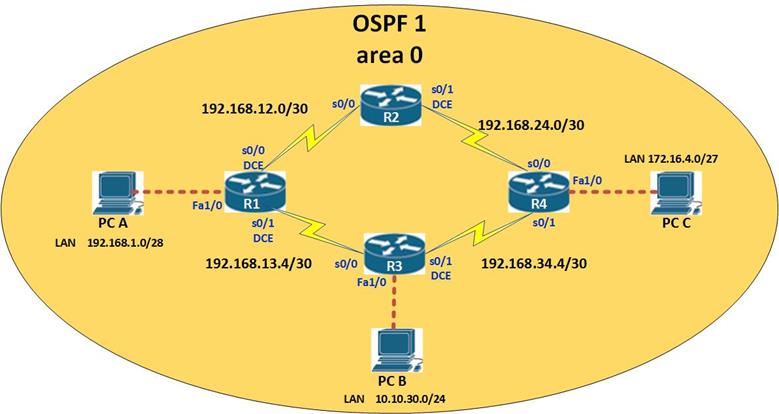
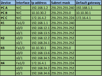
The network consists of 4 routers labeled R1 to R4, there are also 3 LAN segments connected to R1, R3 and R4. The ip subnets in use are shown in the diagram and the ip addressing scheme in use is shown below. The clock rate in use on the DCE interfaces is 64000
Before we begin the OSPFv2 configuration, design the network above and configure the following
- Appropriate host names on all devices
- Appropriate passwords to the console lines and the telnet lines
- Banners
- Disable ip domain lookup
- Ip addresses, subnet masks, default gateways and clock rates appropriately
- Enable the devices and ensure connectivity on directly connected networks
Basic ospf configuration
By now you should be able to do the basic configuration on your own so we will not dwell on it, rather, we will start with the basic OSPF configuration.
Router ospf command.
To enable OSPF on our routers, we need to configure the “router ospf <process-ID>” command in the global configuration mode of our routers.
The process-ID is a logically significant number between 1 and 65535, this number is locally signifcicant which means that it only identifies the OSPF process running on a router. You should note that the OSPF process-ID is not the same as the EIGRP processs ID, thus, neighboring routers do not need this number to match so as to form adjacency.
However, in this course, we recommend that you use the same process ID for consistency.
In our topology, we will use 10 as our process ID on all the routers.
So on R1, we need to execute the command shown below.
R1(config)#router ospf 10
This command allows us to enter the OSPF specific configuration mode. From here, we will be able to configure most of the OSPF options that we need.
The network command
Just like in EIGRP, the network command is used to advertise routes in OSPF, however, the format differs a bit: the network command in OSPF is shown below:
router(config-router)#network <network_address> <wildcard_mask> area <area_ID>
Notice that we have two more parameters, which are the wildcard mask and the area ID.
Area – As we discussed earlier, OSPF uses areas, all the routers in an area usually have the same map. In this chapter, we will only deal with the backbone area which is area 0 this means that all the routers will be in this area.
As the networks grow, the use of multiple-areas is introduced so as to reduce the size of the map. This will be discussed in an upcoming chapter.
NOTE: you must configure the area as “area 0” on all network statements and all routers.
The wildcard mask – or inverse mask is a special type of IP address that is used by OSPF to determine the specific subnet that is being advertised.
Wildcard mask
The wildcard mask is usually the inverse of the subnet mask. To calculate the inverse mask of a network address follow the steps below.
- Write down the subnet mask of 255.255.255.255 which is the broadcast address for any host or the broadcast address of the zero network (global broadcast address)
- Write down the subnet mask of the network or the ip address in question
- Subtract the values of the network’s subnet mask from the subnet mask of 255.255.255.255
This is shown in the table below for the network of 192.168.1.0/27
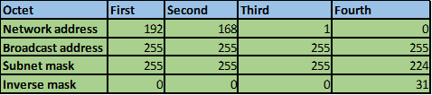
Therefore the inverse mask or wildcard mask for the network 192.168.1.0/27 is 0.0.0.31.
When the router is determining the network it should advertise, a value of “0” will be considered while any value higher than that will be ignored, therefore in the above example, when advertising network 192.168.1.0/27 in OSPF, the first three octets will be considered, while the fourth octet will only be partially considered.
This means that, when the route 192.168.1.0/27 is advertised,
The router will advertise only routes matching the first three octets and ignore the fourth octet.
NOTE: the most specific wildcard mask that can be used to advertise networks in OSPF is 0.0.0.0, which means that the router will advertise only a specific ip address and not a network address.
Just like in EIGRP, we advertise the directly connected networks that we want to participate in OSPF
To advertise the network 192.168.1.0/28 in OSPF, the command we need on R1 is shown below:
R1(config-router)#network 192.168.1.0 0.0.0.15 area 0
Back to the configuration
In our topology therefore, we will advertise all the directly connected networks on each of the routers using the commands shown in the table below.
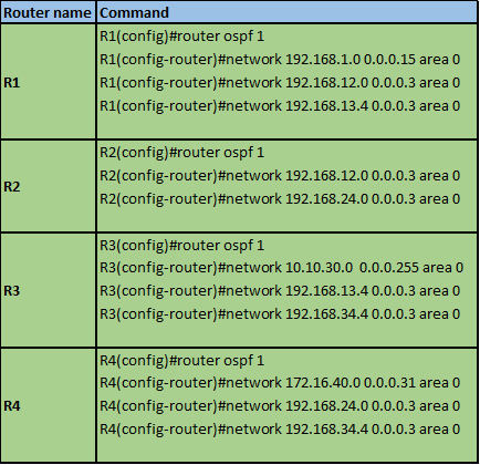
NOTE: When making these configurations make sure that you calculate all the wildcard-masks so that you understand the concept clearly.
After making these configurations you on all the routers you should be able to see the output shown below:
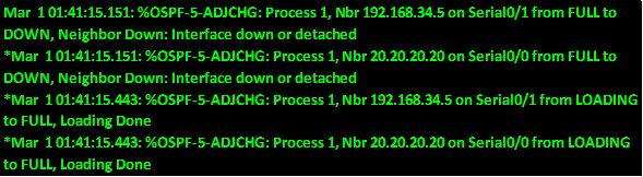
This shows that OSPF is working and all the routes have been learnt. Notice the speed by which this happens, this is how fast OSPF takes to converge.
OSPF Router-ID
In OSPF, the router-ID is a way to name each router in the routing domain. It is simply an ip address that is specially selected to name a router in OSPF. with CISCO routers, the router-ID is selected based on the criteria shown below.
- The IP address configured using the command “router-ID <IP_ADDRESS>” in the OSPF configuration mode.
- If it is not configured, use the highest IP address of any of the configured loopback interfaces.
- If there is no loopback interface, the router uses the highest IP address of any of the ACTIVE physical interfaces.
NOTE: the highest ACTIVE physical interface is an interface that is able to forward packets.
The use and importance of the router ID will be discussed later.
Configuring the router-ID
The router-ID is configured in the OSPF configuration mode which is denoted by the prompt shown below:
Router(config-router)#
The command used to configure the router-ID is:
router(config-router)#router-id <unique_ip_address>
on R1, we will use the ip address 1.1.1.1 as the router-id and this is configured as shown below.
R1(config-router)#router-id 1.1.1.1
When the command above is executed, the router will be set with the manual router-id of 1.1.1.1
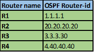
On the four routers, we will use the ip addresses shown in the table below as the router-IDs
Configuring Loopback interfaces
As we mentioned earlier, a loopback interface can be used as the router ID.
A loopback interface is a virtual interface – this means, that it only exists in the router and is not connected to any other physical device in the network. A loopback interface, once configured automatically transitions to UP. The command needed to configure a loopback interface is:
Router(config)#interface <loopback> <Loopback_interface_number>
After executing this command, you will be taken to the interface configuration mode where you can configure other options such as the ip address.
To configure the loopback interface, with an ip address of 172.16.1.1/24 on R1, enter the following command:
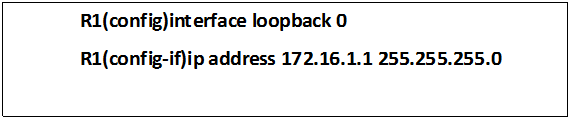
Note: when these commands are executed, a new interface will be shown in the “show ip interface brief”. The loopback interface is always up and operates as a physical interface.
After configuring ospf and saving, the router-ID in use will still be the highest active physical interface that we used, and the router-ID configured using the router-id command will still not be active as shown in the output below.

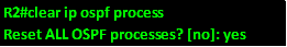
We need to make the router-ID active by restarting the OSPF process on all the routers: to do this, we have to enter the command “clear ip ospf process” in the privileged exec mode as shown below.
Executing this command will prompt us to confirm this command and we should answer with “YES”
After executing this command on all the routers, the new router-ids will be in effect.
Verifying OSPF operation
After configuring OSPF we need to verify that everything is working fine on all the routers. To verify OSPF we will use these commands:
- Show ip ospf neighbor
- Show ip ospf database
- Show ip route
- Show ip ospf interface
- Show ip protocols
- Show ip ospf
- Debug ip ospf adj
- Debug ip ospf hello
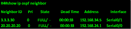
Show ip ospf neighbor
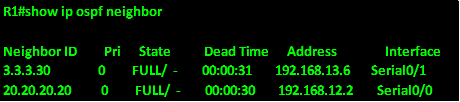
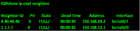
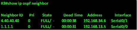
The “show ip ospf neighbor” is top on the list for most useful commands used for verifying and troubleshooting of OSPF neighbor relationships. Some of the information that is displayed using this command is listed below.
- Neighbors’ router ID
- Pri – the OSPF priority
- State – the type of LSA
- Dead time – this is amount of time that OSPF waits until it considers a neighbor as dead as a result of missing hellos.
- Address – neighbors IP address for the shared link
- Interface – the physical interface that a router connects to a neighbor using.
In OSPF for neighboring routers to form adjacency the following conditions must be met.
- The subnet masks used on the links must be the same, meaning that links must be on the same subnet
- Matching OSPF hello and dead timers
- Matching OSPF network types
- Correct network statements
In our scenario, the output of the show ip ospf neighbor on all routers will be as shown below:
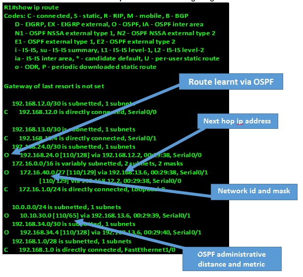
Show ip route
The show ip route command on a router configured with OSPF will show all the routes that the router has learnt, the next hop, administrative distance and metric as well as the age of the routes. The output of this command on R1 will be as shown below.
NOTICE: routes learnt via OSPF show up marked as O at the beginning.
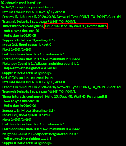
Show ip ospf interface
This command is used to verify the interfaces participating in OSPF as well as the hello and dead timer intervals. It can also be used to show the statistics on a specific interface when the interface name and number are used. The output of this command on R2 is shown below
 .
.
The OSPF hello and dead timers are highlighted in the RED box in the output above. Further, the network type is shown as point to point with a cost of 64.
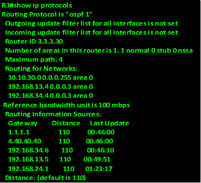
Show ip protocols
The “show ip protocols” command, can be used to verify the routing protocol in use. In this instance, it will show us the OSPF process-ID, router-ID, advertised networks, neighbors, areas and area types, and the OSPF administrative distance.
The output of this command on R3 is shown below.
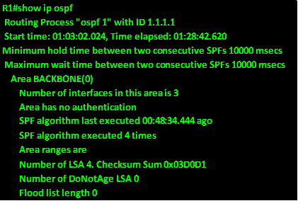
Show ip ospf
The command “show ip ospf” is also a good way to verify the process ID, router IDs, areas, SPF statistics and other information that can be useful in troubleshooting OSPF.
The output of this command on R1 is shown below: Some output from this command has been omitted since it is beyond the scope of this course.
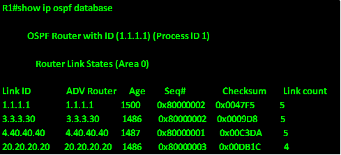
Show ip ospf database
This command will show all the routers in OSPF that have the same OSPF database or “map” if you will. The output of this command on R1 is as shown below.
Other commands that can be used to verify and troubleshoot OSPF are the debug commands. These commands will show statistics of OSPF as they happen and therefore can consume a lot of processing power.
- Debug ip ospf adj
- Debug ip ospf hello
Verify connectivity
After you have configured OSPF on all four routers and verified that all routers have converged and have all the routes, you need to verify connectivity by pinging all the host devices.
- Ping from PC_A to PC_B
- Ping from PC_B to PC_C
- Ping from PC_A to PC_C
If all the pings are successful, you have successfully configured OSPF, if not, follow the steps shown above and try and solve the problem.
End of part 1
With that we have come to the end of part one of OSPF. We have learnt the concepts of LINK STATE routing protocols and especially OSPF, we took at how OSPF works and its advantages. We also configured and verified basic operation of OSPF. In the next part, we will learn more concepts of OSPF and do more configurations.