


Overview
In part 1 and part 2 of this chapter, we looked at the concepts behind OSPF operation. In part three and the last part, which is part four, we will look at more advanced concepts in OSPF. In part three we will look at multi area OSPF. We will learn how it is different from single area OSPF and look at the various concepts behind its operation.
LSA problems
When we were discussing OSPF concepts and the advantages of OSPF over other routing protocols such as OSPF, we saw that in OSPF, the routers maintain a “map” of all the networks in their domain. This is a major advantage over distance vector routing protocols, however, it can be a big problem.
The SPF algorithm is responsible for maintaining the routing information in OSPF, the best routes are calculated based on the routes in the link-state database which is identical on all the routers in the domain. This means that if there is a topology change, the SPF algorithm has to run on all the routers in the domain.
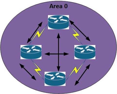
The diagram above, illustrates what happens when OSPF updates are sent to all the routers in an area.
This may not be a big problem in a network that has three or four routers, but can you imagine the effect the SPF algorithm would have on a network with hundreds of routers?
Multi-area OSPF
Multi-area OSPF is a solution to these problems. In this implementation, routers, restrict the Link-state database to their areas, this means that there will be several Link-state databases. One for each area. In turn, SPF calculations are restricted to an area and this eases the load on a router’s resources.
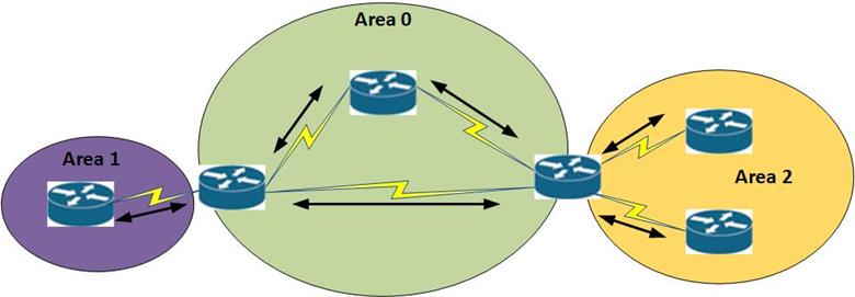
Multi-area OSPF is a way for us to localize the LSA updates to the routers. In the scenario above, the routers in area 0 will have a synchronized Link State Database, the routers in area 1 will also have their own Link-state database as well as those in area 2.
Communication in the network will happen by using summary LSAs to update other areas. This means that the routers in area 1 will send a summary LSA to area 0 and then area 0 will send this summary route to area 2. This is the same as for routers in area 2.
Terminology
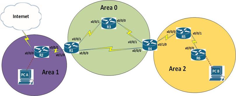
There are several terms that are used to describe the routers in the multi-area OSPF domain. The topology below shows a multi-area OSPF routing domain.
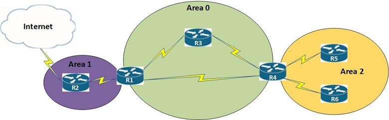
ABR – in the network above, the routers that separate two areas are known as ABRs (Area Boundary Router) in this scenario, R1 and R4 are ABRs. R1 separates area 0 and area 1 while R4 separates area 2 and area 0. An ABR can also be described as a router with interfaces in different areas.
NOTE:
In OSPF we can only summarize networks in the ABRs and ASBRs.
The routers in area 0, are in the backbone area. All the areas must connect to area 0 for communication to happen.
ASBR – an ASBR (Autonomous System Boundary Router) is a router that connects to a different autonomous system. In our scenario above, R2 is an ASBR since one of its interfaces is connected to the internet.
NOTE: in multi-area OSPF, the ABRs must have at least one of their interfaces connected to area 0.
LSA types
A router’s link-state database is made up of Link-State Advertisements (LSAs). There are several types of LSAs in OSPF, these are listed below.
- Type 1 LSA – router LSA
- Type 2 LSA – network LSA
- Type 3 LSA – ABR summary route
- Type 4 LSA – summary LSA ASBR location
- Type 5 LSA – ASBR summary route
NOTE: The use of the different types of LSAs will be discussed in more detail in CCNP.
Configuring multi-area OSPF
In the topology shown below, we have six routers in three areas. Our task is to configure multi-area OSPF and ensure full connectivity on the PCs.
In this lab, successful configuration will be determined when there is end to end connectivity between the hosts.
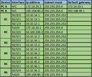
The ip addressing scheme in use is shown below.
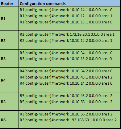
Step 1. Configure the network statements indicating the area of each network
NOTE: a good way to configure ospf networks is to advertise the specific ip address on each interface with a wildcard mask of all “zeros”.
The network statements for this network are shown below.
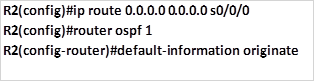
Step 2
After configuring the network statements, we can configure a static default route on R2 and redistribute it.
With this configuration, we should be able to see all the routes. We can examine the routing table of R3 and R6 to see the difference.
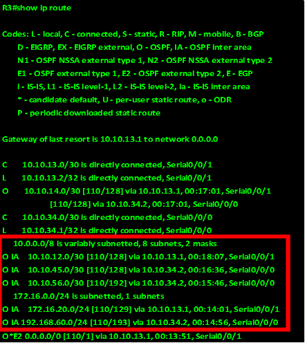
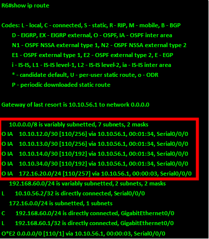
As you can see from both routers, the routes are all present in their routing tables, the inter area routes in these output are marked as OIA – highlighted in red, these are the routes from other areas. The routes marked as O*E2 are external routes. However, if we examine their link state databases, we will note the difference.
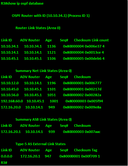
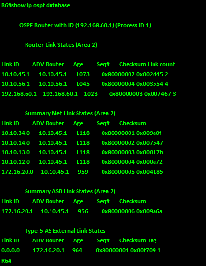
From the output above, you can see that even though R3 has all the routes in its routing table, it only has a link state database with routes in area 0. It receives all other routes marked as type 4 or 5. The same can be said of R6’s OSPF database. It has only the LSA information from routers in area 2. All other information is suppressed at the ABR.
Multi-area OSPF is a very important concept and cannot be discussed fully in this chapter, you will learn more at the CCNP and more advanced levels. However, the concepts that we have discussed here are vital in understanding the operation of OSPF.
Summary
In part three of OSPF, we have looked at configuring multi-area OSPF. We have looked at why it is important and we capped it off with configuring and verifying multi-area OSPF. In part four we will look at other OSPF concepts and configuration.