Dynamic routing protocols

Overview

In the previous chapter, we looked at static routing. We saw how the router finds the best path to a network. We configured static routes and traffic was able to flow between two points.

In this chapter, we will give an overview of dynamic routing protocols. We will define them and learn how they are different from static routes. We will discuss their advantages over static routes, learn the different categories of dynamic routing protocols as well as classless and classful nature. We will also talk about the administrative distance and the metric.

Consider the network diagram shown below.

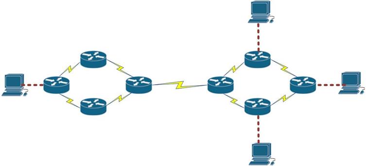
The administrative overhead that would be needed to make communication between all these devices would be considerable. All the static routes would have to be configured.

Wouldn’t it be much easier, for the network administrator to just “Teach” the routers how to get from one point to another? The solution to this problem would be dynamic routing protocols.

Dynamic routing protocols are a solution that is used in large networks so as to reduce the complexity in configuration that would be occasioned by having to configure static routes. In most networks you will see a mix of both dynamic and static routes.

Definition of dynamic routing protocols

Routing protocols are used to enable the routers exchange routing information, they allow routers to learn about remotely connected networks dynamically. This information is then added to their routing tables as a basis for forwarding packets.

Classification

Dynamic routing protocols can be classified in several ways.

• Interior and exterior gateway routing protocols,
• Distance vector, path vector and link state routing protocols,
• Classful and classless.

The table below shows the various categories of dynamic routing protocols and the ones highlighted in red
will be the focus of this course. Others will be discussed at the CCNP and the CCIE level.

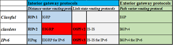
In this course, we will look at EIGRP, OSPFv2 and OSPFv3. These topics will be crucial in passing both your ICND1 and ICND 2 exam, and the CCNA composite exams.

The table below shows more information on the routing protocols to be covered in this course.

Although you may not be examined on the information above directly, both exams will have questions that require knowledge of this information.

Operation of routing protocols

Now that we have an overview of routing protocols, we need to understand how they work.

Routing protocols are comprised of processes, messages and algorithms that are used by routers to learn about remotely connected networks from routers that have been configured with the same routing protocols, the routes that have been learnt are added to the routing table and used as a basis for forwarding packets.

• Routing protocols function by:
• Discovering remote networks
• Maintaining current routing information
• Path determination

The routing protocol is made up of these components.

1. Data structures – this is information about remote networks. It is usually stored in the RAM and may be comprised of tables such as neighbor tables and topology tables.
2. Algorithm – this is the sequential list of steps that the routing takes when determining the best path to a particular network.
3. Routing protocol messages – these are messages that are used to maintain updated routing information. Examples include; hello messages, update messages among others.

The way routing protocols operate may differ depending on the routing protocol, however, there are certain characteristics inherent in every routing protocol.

• Exchange of information on interfaces to discover neighboring routers
• Exchange of routes that have been advertised
• Running of the algorithm so as to determine the best path
• Adding of best paths to the routing table
• Detection of topology changes and making the necessary changes

These are the general steps routers will take. However, the processes differ with each routing protocol and will be discussed at a later stage.

Advantages and disadvantages

Now that we have seen the dynamic routing protocols to be covered in this course, we need to know the advantages and disadvantages of using dynamic routing protocols. We also need to compare them to static routes.

Advantages

• Exchange of routing information when there is a topology change is dynamic.
• Less administrative overhead as compared to static routes which have to be manually configured
• Less error prone than static routing which.
• Scalability, since there is less administrative overhead than static routes.

Disadvantages

• Require more expertise by the administrator, they are not as simple to configure as static routes.
• They use more of the routers resources; such as CPU and RAM.

Egp vs igp

As mentioned earlier, routing protocols fall into two main categories which are;

• EGP – Exterior Gateway Protocols
• IGP – Interior Gateway Protocols

This categorization, is based on the Autonomous Systems.

Autonomous systems also known as routing domains; are collections of routers under the same administration. This may mean the routers that are owned by one company.

For example, company XYZ, could have 1 branch connected to the headquarters through a leased line. The networks owned and managed by XYZ would be one autonomous system, while the leased line and interconnections between the branch office and the headquarters which are controlled by the ISP would be another autonomous system. This is shown in the exhibit below.

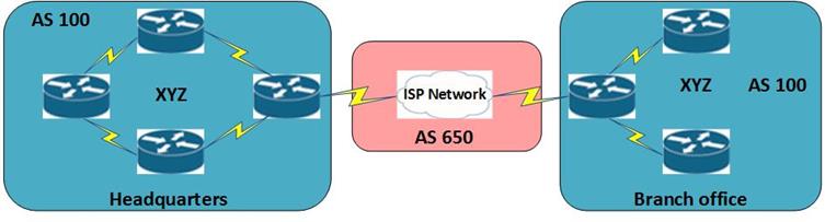
The networks controlled by XYZ are labelled as AS 100 while AS 650 represents the ISP.

Interior Gateway Protocols (IGP) are used for intra-autonomous system routing – routing inside an autonomous system.

Exterior Gateway Protocols (EGP) are used for inter-autonomous system routing – routing between autonomous systems.

In this scenario for example, routing between XYZ headquarters and the branch office would use and IGP, whilst routing between company XYZ and the ISP would use an EGP.

Distance vector routing protocols vs. link state routing protocols

Interior Gateway Protocols (IGPs) can be classified as two types:

• Distance vector routing protocols
• Link-state routing protocols

Distance vector means that routes are advertised as vectors of distance and direction. If we take an example of a tourist getting directions, distance vector protocols would be where the tourist would only use road signs to get to where they are going. They do not know the exact landscape and possible blocks, they only know of the next point towards their destination.

Distance vector protocols work best in situations where:

• The network is simple and flat and does not require a special hierarchical design.
• The administrators do not have enough knowledge to configure and troubleshoot link-state protocols.
• Specific types of networks, such as hub-and-spoke networks, are being implemented.
• Worst-case convergence times in a network are not a concern

On the other hand, if the tourist had an entire map of the desired destination, with details of different paths to where they were going, they would be using a link-state routing protocol.

Link state routing protocols usually have a complete view of the topology. They usually know of the best paths as well as backup paths to networks. Link state protocols use the shortest-path first algorithm to find the best path to a network.

Link-state protocols work best in situations where:

• The network design is hierarchical, usually occurring in large networks.
• The administrators have a good knowledge of the implemented link-state routing protocol.
• Fast convergence of the network is crucial.

Classful and classless

Classful Routing Protocols

Classful routing protocols don’t include the subnet mask in their routing updates. This is because they were designed prior to the introduction of CIDR and VLSM. RIPv1 is an example of such protocols.

Since they do not include the subnet mask in their routing updates, they cannot work where the networks have been subnetted.

Classless routing protocols

Classless routing protocols include the subnet mask with the network address in routing updates.

In this course, we will focus on the classless routing protocols since the use of classful routing protocols is outdated and no longer used in most modern networks.

Administrative distance and metric

Metric

Suppose a router has more than 1 destination to a network, how would it determine the best path to that network?

The metric, is the mechanism used by the routing protocol to assign costs to reach remote networks. In the tourist example, this may be the amount of fuel the tourist has to use to get to their destination. The metric is used to determine the best path to a network when there are multiple paths.

The table below shows the various metrics used by routing protocols which will be covered in this course.

Understanding the different costs types will be crucial in your final exam.

Administrative distance

What if we had configured several routing protocols on one router, how would the router determine the best path to the desired network?

The administrative distance is the way routers use to give preference to routing sources. For example if a router learns of the same route via EIGRP and RIP, it will prefer the route it learnt via EIGRP.

All routes in the routing table are prioritized. With the best and most preferred paths being the directly connected routes. The AD is the trustworthiness of a route.

The AD is usually a value from 0 to 255, the lower the value the better the routing source, a route with an administrative distance of 255 will never be trusted.

If we use the tourist example, the administrative distance would be the trust placed on each means of transport, for example an airline would be more trusted over walking.

The table below shows the various administrative distances for the routing protocols which will be covered in this course.

Summary

In this chapter, we have learnt about dynamic routing protocols. We defined and classified the various routing protocols. We explained how they work as well as their advantages and disadvantages. We also looked at the various classifications of routing protocols such as; EGP and IGP and distance vector and link state routing protocols. We also looked at classful and classless routing protocols as well as explained what the metric and administrative distance mean.

NOTE: The concepts learnt in this chapter are crucial in understanding routing. These concepts are usually examined in both ICND 1 and ICND 2 as well as the CCNA composite exam. These concepts will also be useful at the CCNP and CCIE levels.

In the next chapter, we will look at the first routing of this course which is EIGRP.