Author Archives: ccnablog

Network Security

Overview

In the last chapter, we looked at frame relay and discussed its importance in the WAN. In this chapter, we will look at some network security concepts that are vital in today’s world. We will look at some of the risks as well as the ways we can secure our devices, we will also review security concepts we learnt in previous chapters.

Network security factors

In CCNA, we are supposed to familiarize ourselves with basic network security. The CCNA SECURITY course comprehensively covers the network security concepts that are needed in a small to medium size enterprise. In this chapter, we will look at the three factors that are crucial in networks, we will discuss what vulnerabilities we may have in our networks, the threats that we may face and some of the attacks. These factors are described below.

Vulnerability – this are the weaknesses that we may have in the network. They may be as a result of the technology in use, the configuration on our devices or poor or weak security policies. In our networks, we need to plan for security carefully and consider these factors, a comprehensive security policy would be crucial in ensuring that data in our network is not accessed due to weak security on our devices.
Threats – in network security, anyone who has the skill and the interest to manipulate any of the vulnerabilities, is known as a threat. These individuals or groups may be motivated by many factors such as money, power, and thrill seeking among others. Whatever the motive may be, threats to network security pose a major challenge for administrators since they may access information that is sensitive or even cripple the network.
Attacks – these are the methods that are used by the threats to access the network. There are a number of attacks that can be used to access our network. They may be aimed at the network infrastructure through methods such as dumpster diving, or aimed at users using methods such as social engineering.

Securing the network

The security issues in the network are many and cannot be covered in one chapter, the various methods used by attackers to access networks have grave and far reaching effects, as such, we will focus on protecting routers and switches in this course. Some of the protection methods we will look at include:

Physical security methods
Passwords
SSH
Port security

Physical security

Physical threats to network devices are a major issue. Physical attacks may cripple an enterprise’s productivity due to outage of network services. The four classes of physical threats are:

Hardware threats-damage to network infrastructure such as servers, routers and switches.
Environmental threats– these are the threats that are brought about by storing the networking equipment in unsuitable places; the hardware may be subjected to extreme temperatures or extreme humidity.
Electrical faults – the equipment that is used in our networks relies on electricity to work, as such, any sudden change in the electrical power supplied to the network devices is a major threat.
Maintenance threats – from time to time, we may need to run maintenance checks on our network devices, the use of untrained technicians can pose a major threat to the network devices.

Some of the physical threats may be almost impossible to guard against. For example, we may not be able to predict an earthquake. However, we can effectively mitigate the threats to our network hardware by following the following guidelines:

Hardware threat mitigation

The location used for storing networking equipment as well the wiring closets, should only be accessed by authorized personnel. All the entrances should be secured and monitoring should be implemented by using CCTV cameras.

Environmental threat mitigation

The environment should be controlled to mitigate the environmental factors. the humidity, temperature, and other environmental factors should be monitored. The network control room should ideally be in a room where the conditions can be controlled effectively.

Electrical threat mitigation

The electrical threats may be mitigated by using UPS systems, so that the networking devices don’t draw their power directly from the mains. There should be backup systems such as generators and inverters so as to maintain network connectivity in case of power outage.

Maintenance threat mitigation

Maintenance threats should be mitigated by using well trained personnel. All the cables should be well labeled, maintenance logs should be maintained, and there should be availability of spare parts that are critical to maintaining connectivity.

Passwords

In the previous chapters, we discussed how passwords can be used to protect network devices, we looked at limiting access to the router and switch, console lines and telnet lines.

NOTE: passwords should be limited to administrators only, they should not be written down and should be changed regularly. A good password should contain a variety of characters.

Use of encrypted passwords is also better than passwords that have been stored in plain text.

SSH (secure shell)

We learnt that we can manage our routers and switches either locally using console and auxiliary ports on the router or remotely using virtual terminal lines.

Local access is the more secure way we can configure our routers, however, in some cases, we may not be able to access the network through the console port. For example, you may need to troubleshoot an issue on a router while you are on a trip.

Remote access gives us a more convenient way to manage an attacker, however, this may increase the vulnerability. For example, if we use plain text passwords, an attacker may capture packets that reveal the password.

Telnet is one way we can configure a network remotely, however, it is insecure since traffic is not usually encrypted. As such, we need to use a different protocol that will enable us to configure our network devices remotely in a secure manner.

The SSH protocol, is a management protocol that enables us to configure our devices securely in place of telnet. This protocol uses the TCP port 22.

We can use SSH to accomplish the following:

Connect to the virtual terminal lines on a router so as to configure other devices securely
Connect remotely and securely to a terminal server so as to make a specific configuration change
Connect to modems attached to routers by dialing out securely
Authenticate when making configuration changes by requiring passwords and usernames for each configuration line

Configuring SSH on Virtual terminal Lines

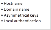
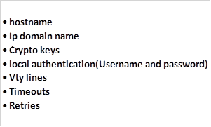
To enable SSH on a router, we must configure the following parameters.

We can also configure the following optional configuration parameters:

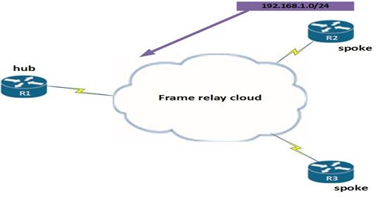
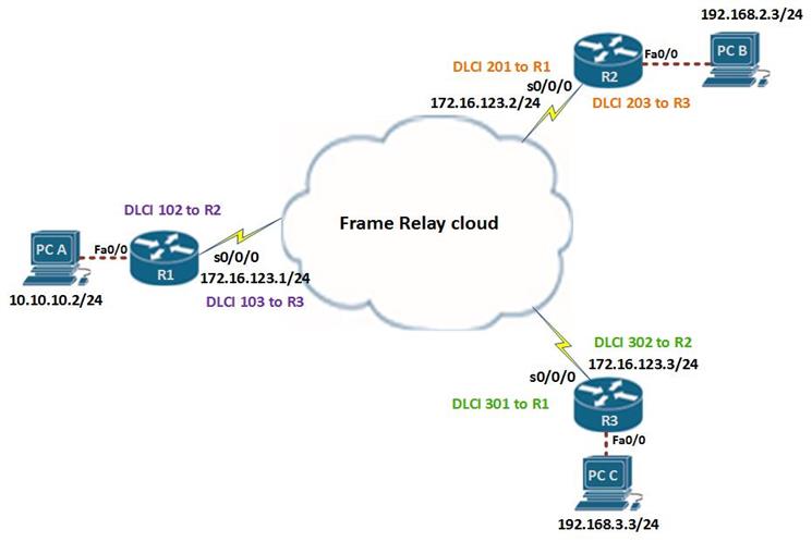
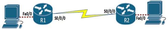
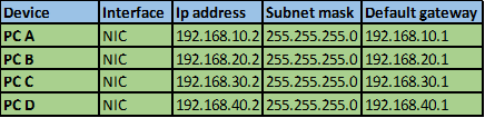
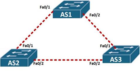
The diagram shown below shows the topology that we will use in this lab. The ip addressing has been configured and our task is to configure SSH on R2 so that users on R1 can only access it securely.

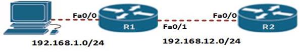
In this scenario, we will only be configuring R2 and the success of this lab will be determined when R1 can be able to access the console line of R2. Our configuration items include:

Step 1. Configure hostname

We need to configure the hostname to be used by the router using the command shown below in the global configuration mode.

Step 2: configure domain name

For SSH to work, we need to have a domain name. The command needed to configure a domain name is:

In our scenario, this command is implemented as shown below for a domain name called “cisco.com”

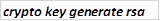
Step 3: Generation of the asymmetric keys

In SSH, we need to create a set of encryption keys that will be used to encrypt the SSH traffic. This is implemented in the global configuration mode using the command:

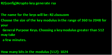
When this command is executed in a router, we are prompted to enter the size of the keys within a range of 360bits to 2048 bits. The longer the key the better the encryption, however, the longer our key the longer the time needed to create them.

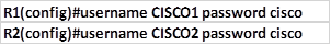
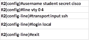
Step 4: the last compulsory configuration, is configuration of the local authentication which is done by configuring the username and a secret.

This is followed by implementing the SSH protocol on the virtual terminal lines. In our scenario, the username we will use is: “student” with the secret “cisco“. To activate SSH in the vty lines, we use these commands in the vty lines configuration mode:

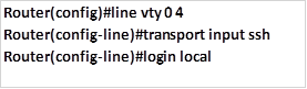
The command shown above, specifies that we are configuring 5 vty lines for SSH with the login mechanism being the local username and secret. The implementation of these commands in our scenario is shown below.

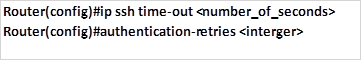
Step 5: Configure SSH timeouts (optional)

We can also specify the number of times that a person can try entering a password as well as how long they would have to wait if they get it wrong. This is optional and it is implemented using the commands shown below:

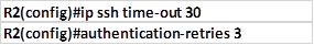
In our lab the SSH timeout is set to 30 seconds and the amount of retries to 3.

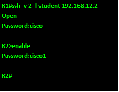
To test the remote terminal line connection, from R1, we use the following command:

The “-V” keyword specifies the version of configured on the remote router.

The username, and ip address or domain name are the remote router’s configured username and password.

After entering this command, you will be prompted for password for the SSH line.

After entering the VTY password you will be prompted for the router’s password and successful entry will gain you access.

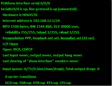
The output below shows the access procedures for accessing R2 from R1.

NOTE: the passwords in this output have been shown but when accessing a real router, they will not be shown, and therefore it is imperative that you type in the password correctly.

NOTE: the process of login in remotely is a very important aspect and it is frequently asked in CCNA exams. It is therefore vital that you understand the security procedures for accessing a remote router.

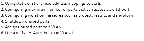
Port security

Port security is important in switch security. Unused ports are a major security issue since they can be used to attack the network. As discussed in the chapter on switch operation, securing switchports includes:

NOTE: the security concepts in CCNA are many and they are mostly covered in the security course, however, these concepts are crucial in securing a network.

Summary

In this chapter, we have looked at some of the security issues that affect the network, we discussed the security factors as well as the threats to network security. We then looked at various methods of securing the network and configured SSH as an alternative to telnet. In the next chapter, we will look at access control lists and discuss how they help in networks by adding security and traffic filtering.

Frame Relay – Part II

Overview

In part one of this chapter, we looked at the concepts behind frame relay operation. We discussed the role of the PVC’s, DLCI mapping, inverse ARP among other topics. In part two of this chapter, we will discuss more advanced frame relay concepts and finally look at the commands used to troubleshoot frame relay.

Advanced frame relay concepts

Split horizon

In NBMA networks, the topology used is mainly hub-and-spoke. This means that when we use routing protocols, we can have issues with reachability due to split horizon.

If you can recall, Split horizon prevents a router from advertising routes out the interface it learnt them from.

In the example shown below, R2 advertises the route 192.168.1.0/24, to R1. When R1 – the hub of the network receives this route, it has to advertise it to R3 so that the network can be converged, however, it cannot do this since there is only 1 interface and split horizon prevents it from advertising the route 192.168.1.0/24 to R3 out the same interface.

Subinterfaces

Recall we said that subinterfaces are virtual interfaces that are configured on a physical interfaces.

To avoid split horizon in frame relay, we can divide the physical interface using subinterfaces that connect to different subnets. With this, we can have two types of implementation; point-to-point, where 2 points use one network address, or point-to-multipoint, where more than 2 points use 1 subnet.

This would resolve the split horizon issue since the packets received on a physical interfaces are considered to be in a different interface which is the subinterface. This means that the same physical interface can then forward the packets out through another subinterfaces.

Frame Relay subinterfaces can be either point-to-point or multipoint mode:

Configuring subinterfaces

Step 1. to configure the subinterfaces, we first need to remove any layer three addresses that may have been configured physical interface. This is because the physical interface will be used by the subinterface and if it has a layer three address, the frames will not be received. To accomplish this, we can use the “no ip address” command in the interface configuration mode for the interface that is connected to the frame relay cloud.

Step 2. The configuration that is needed on the physical interface is the encapsulation command for frame relay as well as the activation of the interface using the “no shutdown” command. Step one and two are implemented as shown below.

Step 3. The third step is the most vital. We need to create subinterfaces for each of the Virtual Circuits in the frame relay cloud. The creation of the subinterface is done using the command shown below.

When configuring the subinterface, do not forget the period (.) between the interface ID and the subinterface ID. Which is our example above is shown in red.

NOTE: as good practice, when configuring subinterfaces, you are adviced to use a subinterface number that is the same as the DLCI number for that network. This makes it easier to troubleshoot when there is a problem.

When this command is executed, the prompt will take us into the subinterface configuration mode which is denoted by the prompt shown below.

Step 4. The fourth task is to configure the layer three address that will be used for the particular network.

Step 5. The fifth and final task is to map the DLCIs to the specific subinterface. This is shown below.

with this configuration, we will be able to use routing without the problems associated with split horizon.

NOTE: the concepts in frame relay subinterfaces will be explored in more detail in more advanced courses such as CCNP, however, it is important to know these concepts since they are usually examined in the CCNA exams.

Other frame relay concepts

The final concepts that we will look at in this chapter are the payment options in frame relay networks. These concepts are vital in the real world where you may be required to review the service levels of the WAN.

Port speed – this is the speed at which the customer views the connection to the frame relay cloud. In most cases, this is the actual wire speed.

CIR (Committed Information Rate) – this is the actual speed of data transfer that the customer pays the WAN provider for over the frame relay link.

Bursting – in frame relay, if the network is not overloaded, the excess bandwidth is usually shared among the clients in the frame relay cloud without additional cost. This means that data can flow at speeds above the CIR.

Frame relay congestion – in frame relay, the routers can be notified of congestion. These mechanisms are meant to minimize the impact of a congested link. The two notifications that are sent are the:

FECN – Forward Explicit Congestion Notification
BECN – Backward Explicit Congestion Notification

When there is congestion in the network, the frame relay provider uses the following rules to frames that are sent to the frame relay cloud.

To view these statistics on the router, the command needed is:

Troubleshooting frame relay

There are several commands that can be used to troubleshoot frame relay. Most of these we have discussed when configuring frame relay. The commands listed below are key in troubleshooting and verifying frame relay operation.

Show interface serial <interface_ID>

This command shows the operational status of the interface, the bandwith, the LMI type as well as the encapsulation that is in use, the output of this command on R1 is shown below.

Show frame-relay map

This command shows the various frame relay maps whether dynamic or static, it can also be used to check the inverse arp processes on a router. The output of this command is shown in the example below.

If there are no mappings for frame relay, it is advisable to check the configuration made using the command “show running-config”

Show frame-relay pvc

As mentioned earlier, this command shows the status and statistics of the various PVCs on the router.

This command is also useful for viewing the number of BECN and FECN packets received by the router. The PVC status can be active, inactive, or deleted.

The “show frame-relay pvc” command displays the status of all the PVCs configured on the router. The output of this command is shown below.

Show frame-relay lmi

The “show frame-relay lmi” command helps isolate the problem to a Frame Relay communications issue between the carrier’s switch and your router. Look for any non-zero “Invalid” items. The output of this command is shown below.

Debug frame-relay lmi

To find out if the router which is the DTE device and the frame relay switch which is the DCE are communicating properly through LMI packets, we can use the command “debug frame-relay lmi“. This is the last command that we will discuss in this chapter. The output of this command is shown below.

The meaning of the keywords in this output is shown below:

“out” at the end of the interface denotes LMI status messages sent out of the s0/0/0 interface of this router.
Messages that are received from the frame relay cloud are denoted by “in” at the end of the interface ID
“type 0” denotes a full LMI status message
“type 1” denotes an LMI exchange.
“dlci 102, status 0x2” means that DLCI 102 is in active state.

The connection states made by a router as a result of inverse ARP requests are three. These are shown below.

ACTIVE – full connectivity on the PVC, both the remote and local router are connected.
INACTIVE – the connection to the frame relay switch is active, but the remote router is not connected to the frame relay cloud.
DELETED – denotes that the router is configured with an invalid DLCI

The possible values of the status field are as follows:

0x0 – the DLCI has been configured but the PVC is unusable
0x2 – full connectivity
0x4 – the frame relay switch has not been configured with the specific DLCI; it has either been removed by the WAN provider or deleted on the DTE device

NOTE: the debug frame-relay lmi command can be very useful in troubleshooting a frame relay connection, however, debugging commands are usually resource intensive and thus they can affect the router’s performance. It is important to understand these verification and troubleshooting commands since they form a large part of question on WANs in the CCNA exams.

Summary

With the troubleshooting of frame relay section complete, we have come to the end of this chapter on frame relay, as well as the topics on WANs, in this chapter, we have looked at the frame-relay concepts, configuration and troubleshooting.

In the next chapter, we will discuss network security concepts.

Frame Relay Part I

Overview

In the previous chapter, we looked at PPP, we discussed how PPP worked and we said that it works at the data link layer, in this chapter, we will look at the final WAN topic in this course which is frame relay. In part 1, we will discuss the concepts behind frame relay operation as well as the terminologies used we will then configure basic frame relay. In part two, we will look at more advanced frame relay concepts as well as troubleshooting commands.

Introduction to frame relay

Frame Relay is WAN protocol with high performance operating at layer 1 and layer 2 of the OSI model. In frame relay, costs are reduced by using less equipment, easy implementation and reduced complexity, despite this, it is possible for a customer to get high bandwidth, reliability and more resilience as compared to leased connections.

Frame Relay Operation

In frame relay, the connection from DTE to the DCE devices, is made up of both physical layer components as well as data link layer components.

In frame relay, the routers connected to remote networks are usually the DTE devices while the frame relay switch is usually the DCE device. The frame relay switches move data frames from the host networks across the WAN network to the remote DTE devices.

The diagram below shows how this works.

The DTE devices which are the routers, send data from the host network to the frame relay device which is the DCE device the DTE is connected to, then the frame relay switches which are the DCE devices, send the data to the DCE on the edge of the destination network, the data is then sent to the DTE devices on the destination network.

Virtual Circuits

In frame relay, the connection between the two remote DTE devices is known as a (VC) virtual circuit. Unlike direct connections such as PPP and HDLC, there is no physical connection between the host and destination networks between the frame relay networks.

The Virtual Circuits are used as a path for bidirectional communication between the source and destination devices. They are identified by addresses known as DLCIs which are usually given out by the WAN service provider.

The DLCIs in frame relay are only significant in the host network or locally. This means that they are usually not unique in the frame relay network. They usually identify the virtual circuit to the equipment at the end of the frame relay circuit. This means that we can have devices connected by the same Virtual Circuit using different DLCI values.

In the figure below, you can see that R1 has a DLCI to R2 which is 102, however, this changes when it gets to the frame relay network. This is also the same for DLCI 203 on R2 to R3. This shows that DLCIs are only significant locally.

For data to be transmitted in a frame relay network, CISCO routers must know the DLCI value that is mapped to a network layer address towards the destination. The mapping of DLCIs to layer three addresses is accomplished either using static mapping or dynamic mapping.

Inverse ARP

Inverse ARP, is a protocol that resolves or obtains layer three addresses of routers in other networks from the layer two addresses – which are the DLCIs. the Virtual circuit can only be used if the layer 2 addresses are resolved to the layer 3 addresses.

Dynamic Mapping

Dynamic mapping of addresses in frame relay uses inverse ARP to figure out the network layer protocol address that is mapped to a local DLCI. A router in frame relay requests the layer 3 addresses by sending inverse ARP messages out of its PVC. When the frame relay switch responds, the router makes mappings of the DLCI values it gets to layer 3 addresses.

NOTE: inverse ARP is usually on by default on the physical interfaces on a CISCO router for all the layer 3 protocols that have been configured. This means that if you only use IP then the inverse ARP will only work for IP.

LMI Local Management Interface

The LMI is a mechanism that provides information on the status of a frame relay connection between a DTE and a DCE device. This means that it tells the DTE if the frame relay connection is still active by sending out messages every 10 seconds. If the frame relay switch does not respond, the connection is considered as down.

There are several LMI types, and they are incompatible with others, the LMI configured must match the LMI on the service provider. In this course, we will be using two LMI types which are:

Cisco – Original LMI extension
Ansi – Corresponding to the ANSI standard

Basic frame relay configuration

In this section, we are going to configure basic frame relay operation using the topology shown below. The configuration for the frame relay switch is not up to you and it has been done. Our tasks are shown below.

Enable frame relay encapsulation
Configure static and dynamic address maps
Configure the LMI

The LAN interfaces on the routers have been configured with the first viable ip address on the subnet they are on, the serial interfaces have been configured with the ip addresses shown in the topology diagram above. The basic configuration on this lab has been done, and as such our task will be limited to the listed configuration items only. The success of this lab will be when the connectivity of the network is full and all the PC’s can ping each other. The routers have also been configured with EIGRP, therefore there will be layer 3 connectivity.

Step 1. Configure frame relay encapsulation on the serial interfaces.

The command needed to configure frame relay encapsulation on serial interfaces is:

On our three routers, we need to execute the command above and activate the interfaces using the “no shutdown” command as shown below.

NOTE: when configuring encapsulation, there are two options we can use either cisco or ietf, the default option on CISCO routers is “cisco”. If our network has routers from other brands, then we need to use the “ietf” encapsulation.

This will change the encapsulation from HDLC to frame relay, and this can be verified using the “show interface serial <interface_ID>” command as shown in the output below from R1.

As you can see from the output, the interface is line protocol down, this means that it is not yet active.

Step 2. Bandwidth

We can configure the bandwidth which will be used by the routing protocols such as EIGRP and OSPF when calculating the metric. To configure the bandwidth we use the command “bandwidth <number_in_kb/s>” in the interface configuration mode. The commands needed to set up bandwidth of 64kb/s on the serial interfaces on the three routers are shown below.

Step 3. LMI type

This is an optional configuration command and it specifies the LMI type to be used whether cisco or ansi. The command needed to accomplish this is shown below.

In our scenario we will use the cisco LMI type and it the configuration lines needed in the serial interfaces are shown below.

Step 4. Configure static frame relay maps

CISCO routers can use a variety of layer 3 protocols in frame relay. The task of the administrator is to configure the mapping for the layer 3 to layer 2 addresses used in frame relay. This means mapping a layer 3 address such as IP addresses to DLCIs. This can be done either dynamically or statically.

Static frame relay maps are usually configured manually on the router. The command needed to make the static mapping of a network layer address and a DLCI address is:

This means, to get to that ip address, use this DLCI on my router.

Frame Relay, is an NBMA network, this means that it doesn’t support multicast messages or broadcast messages. Therefore, in these networks, we cannot use routing protocols without additional configuration. The broadcast keyword used when configuring the frame relay maps is used for this.

When the “broadcast” keyword is used in the map, the packets that are needed to make routing possible are turned to unicast messages directed to each destination router in frame relay.

NOTE: routing will not occur if the broadcast keyword is missing in the frame relay map command.

The topology diagram shows us the mapping addresses that will be used in this lab, and the table below shows the frame relay map commands that should be used in this lab.

To verify the static frame relay mapping use the command: “show frame-relay map” on each of the routers as shown below for R1 and R3.

Testing connectivity on our hosts is the last thing we need to do in this lab, we can verify that all the three routers have the routes learnt via EIGRP as shown from the output of R3 below.

We can also verify connectivity by pinging from PC A to PC B and as you can see from the output below, the pings are successful.

This marks the end of the first lab, in the next section we will learn more advanced frame relay concepts and finish off with the troubleshooting section.

Summary

This is the end of part one of this chapter on frame relay. In part two, we will learn some more advanced concepts such as split horizon and subinterfaces in frame relay as well as learn the commands that can be used to troubleshoot frame relay.

PPP (Point-to-Point Protocol)

Introduction

In the previous chapter, we discussed serial connections in the WAN, we also discussed the default data link encapsulation on CISCO switches which is HDLC. In this chapter, we will look at PPP, we will discuss some of its concepts, learn how to configure PPP as well as its authentication options and finally we will look at verification and troubleshooting of PPP.

PPP explained

PPP is a WAN protocol that works at layer 2 by encapsulating frames for transmission over a variety of physical links such as serial cables, cell phones, fiber optic cable among others. it offers many more features as compared to HDLC and it is an open standard. Some of the features that it offers which are not available in HDLC include:

Link quality management which is a way to monitor the quality of a link in PPP. When PPP detects too many errors on a link, the link is shut down.
Authentication using PAP and/or CHAP

PPP operation is made using three parameters:

Encapsulation of frames using HDLC protocol
LCP (Link Control Protocol) for establishment, configuration and testing of the link
NCP (Network Control Protocols) to negotiate the different layer 3 protocols.

Link Control Protocol (LCP)

This is the main protocol that PPP uses for its operation. LCP works on top of layer 1 and it works by establishing, testing and configuring the physical connection. It also negotiates other WAN options that are handled by the NCPs. LCP configures the link in the ways listed below:

Determining transmission of different packet sizes
Detection of misconfiguration errors
Termination of the link
Determination of link failure

LCP is also used to negotiate encapsulation parameters and other PPP configuration options such as authentication, error detection and compression when the link has been established.

Network Control Protocol Layer

NCPs are protocols that allow PPP to use different layer 3 protocols such as IP, IPX and Apple Talk.

Establishing a PPP Session

When establishing a PPP session, LCP negotiates the PPP configuration options at either point of the link. This is completed when acknowledgment frames are sent.

The second step is usually optional and it is where LCP tests the link to ascertain whether it has the needed quality to support the various layer 3 protocols.

Finally, NCP is used to configure the layer 3 protocols that are in use.

Configuring PPP

Now that we have learnt the workings of PPP, we can go ahead and configure it. The figure below shows the topology that we will be using in the configuration of PPP.

In our lab, all the options for the PCs as well as the interfaces connecting to the routers from the PCs are configured. The routers have been correctly configured and our task is only to configure the PPP options on the serial links.

The lab requires that we configure basic PPP and successful completion of the lab will be determined by the verification commands we learnt earlier.

NOTE: the routers you will use should have serial interfaces.

Encapsulation

The main command used to enable PPP is: “encapsulation ppp” command. This command should be entered in the serial interface of the routers as shown below.

The command shown above does not have any other options, however, to use PPP, you must have a layer 3 protocol.

In our scenario, all we need to do is to enter this command on the serial interfaces of R1 and R2 as shown below.

Link quality percentage

As we mentioned earlier, the quality of a link is crucial to PPP. The link quality percentage configuration parameter is used to set the baseline quality percentage. When the link does not meet the specified quality, PPP does not activate the link.

The link quality is usually maintained by a parameter called LQM (Link Quality Monitoring) which uses a time lag to make sure that the line does not fluctuate.

To implement link quality percentage as a requirement for PPP establishment, we use the command: “ppp quality <PERCENTAGE>” in the interface configuration mode, this is shown below for our scenario.

This will ensure that the link meets this threshold for PPP to work.

Multilink PPP

Multilink PPP is a way to use many physical WAN links with PPP. This in effect allows for load balancing.

The command for configuring multilink PPP is: “ppp multilink” in the interface configuration mode as shown below for R1 and R2.

NOTE: the quality and multilink commands are not frequently used, and they may not work on Packet tracer simulator.

Verification of ppp

To verify PPP configuration, the “show interface serial <interface_ID>”, “show interfaces” and “debug ppp” commands are mostly used. In this course however, we will mainly use the “show interfaces <interface_ID>” command, the output of this command is shown below.

As you can see from the output of this command on R1, the interface is up and connected – shown in the yellow box, and the encapsulation is shown as PPP (HIGLIGHTED IN RED).

NOTE: the interface status is one of the most important diagnostic features of serial interfaces as discussed in the previous chapter. The debug commands will give live updates for ppp on the router they are issued.

PPP authentication

In PPP, we can secure communication between two points using authentication. There are two ways in which we can configure PPP authentication as discussed below.

PAP (Password Authentication Protocol)

In this form of authentication, the username and password are usually sent in plain text. The central site initiates the authentication by sending a username and a password. The remote site can then reply by either accepting the authentication if the parameters are correct or rejecting it.

CHAP (Challenge-Handshake Authentication Protocol)

In this type of authentication, the remote router sends a challenge to a router that is trying to communicate. The router then responds with an encrypted username and password and if the parameters are correct, the remote router accepts the PPP connection.

The figure below shows the two authentication processes on two routers.

Configuring ppp authentication

The command to enable authentication in PPP is “ppp authentication <pap/chap>“,You can enable both methods of authentication or either of the two.

To configure PAP, the command we use in the interface configuration mode is:

This is followed by specifying the username and password that will be used for authentication as shown below.

On our routers, the commands needed to configure PAP are shown below.

NOTE: The PAP username and password that each router sends must match those specified with the username name password password command of the other router. This is configured using the command “username <username_WORD> password <password>” in the global configuration mode as shown below for R1 and R2.

REMEMBER: the username and password used in ppp authentication in the routers interface should be the username and the password for the other router as configured in the global configuration mode.

You may enable PAP or CHAP or both. If both methods are enabled, the first method specified is requested during link negotiation. If the peer suggests using the second method or simply refuses the first method, the second method is tried. To enable both the command “ppp authentication” should be followed up with the authentication methods you would like to apply, in the order of preference.

For example if we wanted to use CHAP first then PAP, we would need to enter the command shown below.

To enable CHAP, the commands needed are slightly different.

NOTE: The hostname on one router must match the username the other router has configured. The passwords must also match.

Verification and troubleshooting ppp

PPP configuration can be especially challenging. The ppp authentication options are especially tricky, therefore it is imperative that you follow these guidelines very carefully.

To troubleshoot ppp, we can use the various show commands as well as debug commands. The commands for troubleshooting are listed below.

Show interface serial <INTERFACE_ID>
Show interface
Debug ppp

NOTE: the debug ppp command has other keywords that may be used.Make sure you turn off debugging of ppp using “undebug ppp” or “undebug all”, since debugging is resource intensive and can affect performance of the router.

The output of the “show interface serial” <interface_ID> for the serial interface on R1 Is shown below.

With the output of this command, we have completed our topic on PPP. Be careful when it comes to PPP authentication since it is a very important element in understanding PPP.

Summary

In this chapter, we have looked at PPP protocol and how it fits in the WAN, we looked at some of the concepts such as the LCP and NCP as well as the PPP session, we then configured PPP as well as some of its options such as quality and load balancing on numerous links, we then configured PPP authentication using PAP and CHAP and concluded with verification and troubleshooting of PPP. In the next chapter, we will look at frame relay and discuss its importance in the WAN environment.

Serial Connections and HDLC

Introduction

In the last chapter, we discussed some of the concepts that make the WAN work, we briefly described some of the protocols in the WAN. In this chapter, we will discuss serial links and the physical connections we use. We will then explore the default encapsulation on CISCO routers which is HDLC and finally discuss how to troubleshoot a serial connection.

How serial communications work

When communicating data, there are two types of transmissions that can be used; parallel and serial communication. In our computers, the distance between two points is short and therefore parallel communication is used. When the distance increases, we use serial communication whereby the electrical signals are converted to a form that can be transmitted over serial links.

The figure below shows the difference between serial and parallel transmission of data.

In serial communication, we can have only 1 bit transmitting at a time, while parallel communication the communication is much more efficient. However, timing in parallel communication means that all the bits must arrive at the destination at the same time. This is a major problem when communication is happening over long distances.

In our example above, the parallel line can send 6 times as many bits as the serial connection therefore it is theoretically faster. The reason as to why this is the case is due to the fact that parallel communication need clocking to synchronize the arrival time of the bits. The stream must wait until all bits arrive for a full byte to be transmitted.

Communication over serial connections requires fewer cables and wires as compared to that of parallel communications. These cables are also better insulated from noise and other forms of interference.

With parallel cables, the bundling can cause crosstalk and noise.

When using serial cables, the routers and other internetwork devices usually compensate for crosstalk before transmission of the bits. Therefore, the communication using serial cables is more efficient and can operate at higher frequencies.

Serial connection standards

In the previous chapter, we briefly discussed the various types of connectors used in the WAN. In the previously section we have seen that serial connections are less vulnerable to crosstalk, and since they require less wires, they are cheap to implement. This makes them ideal for WAN communications.

The different standards used in serial communications use one of three standards when connecting LANs to the WAN. These are described below.

RS-232 – this standard uses either 9 pin or 25 pin connectors. They are used in serial connections for a variety of purposes and not just limited to WAN connections. Some of the ways they are used include; connection of PCs to printers, modems and other devices.

This is the port that we use to configure a router from the PC. The figure below shows the connector that is used.

V.35 – this is the ITU standard for high speed serial communications. It combines the bandwidth of available on a couple of telephone circuits. This cable is used to connect the DTE devices to modems and similar digital line devices.

High Speed Serial Interface (HSSI) – this standard supports speeds of up to 52Mbps, it can be used to connect LANs to WANs using high speed links such as the T3 lines.

TDM (Time Division Multiplexing)

Time division multiplexing is a technique employed in serial communications to split the bandwidth into slots so that simultaneous communication can happen between several devices. It was a technique first employed by Bell Laboratories to maximize the amount of voice traffic carried over a medium. Prior to the introduction of this technology, telephone calls required dedicated physical links from the source to the destination which was expensive to implement.

In the figure below, we have demonstrated TDM using three conversations over a network, web browsing denoted by “H” voice traffic denoted by “V” and video conferencing denoted by “C”. Notice that the medium is not only carrying one type of traffic, rather it is splitting the communication streams. The recipient rarely sees this happening since the communication is reassembled at the destination.

In serial transmissions, the use of TDM is used as a way to use the bandwidth more effectively. With this communication, the data is reassembled by the destination device.

When the source sends data, the data is split according to the type of protocol as shown above. The data is then transmitted in slots over the physical medium. When the data reaches the destination, the destination device reassembles the data into the specific protocols.

NOTE: in the above example, voice has been given first priority then video finally http data. This is typical in communication and it a principle under QOS (Quality Of Service) this will be discussed in more detail at the CCNP level and above.

DTE-DCE

The communication through the WAN is through the DTE and the DCE device. A serial link is usually made up of two DCE devices at each end. The DCEs connect to DTEs in the remote LAN networks.

The DTE is usually a router or similar device. This is usually the source of the information at a layer 2 perspective. The DTE usually sends the data to the DCE.

The DCE which in the scenario shown below is a CSU/DSU device, converts the data received from the DTE device into a form that can be transmitted over the WAN provider using the serial link. When the signal is received by the DCE at the remote network, it is converted to a form that can be used by the DTE which delivers the data to the destination device.

This is illustrated below.

The DTE in networks is usually owned and maintained by the customer while the DCE devices are usually maintained by the WAN service provider.

NOTE: a CSU/DSU converts digital signals into a form that can be understood by the DTE, in analog signals, a modem is used as a CSU/DSU. In our labs, we do not use the CSU/DSU rather we simulate them using the V. 35. Serial connection with one male side as the DTE and the female side as the DCE.

WAN Encapsulation Protocols

In the WAN environment, we need to specify the particular protocol that the DTE should use. This is so as to make sure that the frames that are sent over the WAN link are correct. The choice of WAN protocol can be determined by a couple of factors.

Below, we have described the various WAN protocols that we will cover in this course.

HDLC – on point-to-point networks, this is the default WAN protocol that is used by CISCO devices. It also defines some of the communication parameters used in PPP.
PPP – is a protocols that connects many routers to the WAN, PPP is works at layer 2 and is independent of the Layer 3 protocol in use. This means that it can use IP, IPX and appletalk.
Frame relay – is an industry standard switched data link protocol. It uses virtual circuits and it evolved from the X.25 protocol. It is more efficient and does not include options such as flow control and error control.

HDLC

This protocol is defined by ISO and it is therefore an open standard. HDLC uses synchronous serial transmission for error free communication between two devices.

HDLC is the default serial links layer 2 protocol and it is enabled by default. However, to configure HDLC on a router’s serial interface, the command: “encapsulation hdlc” is all that is needed.

To verify the encapsulation type on a CISCO router, the command needed is:

The output should show you the encapsulation type as shown in the output below highlighted in red.

Troubleshooting serial interfaces

Troubleshooting a serial interface is a very important aspect in understanding WAN communication, in the output above – highlighted in yellow, the status of the physical layer and data link layer are shown. In the table below, the various messages for the physical layer status and data link layer status are shown and they describe what to look for in every message.

NOTE: these steps are very vital in passing the CCNA exams and are often asked, therefore it is imperative that you understand each message and the problems associated with it.

Summary

In this chapter, we have discussed serial interfaces in detail, we discussed how communication over serial links works as well as the types of serial links. We discussed the use of the DTE and DCE and then we looked at the default WAN encapsulation on CISCO routers which is HDLC. We finalized by learning how to troubleshoot serial interfaces. In the next chapter, we will look at the second serial connection protocol which is PPP (Point-to-Point Protocol).

Introduction to WANs

Introduction

In the previous chapters, we have been primarily focused on LAN technologies, however, as an enterprise grows, so does its networking needs. Consider company ABC, they formed in 2010 in New York, however, over the last couple of years they have grown rapidly and they now have three branches, one in Los Angeles, Miami and they recently diversified into London.

LANs would not be viable for communication over the four geographical information, and therefore there is need for WANs to be incorporated. In the next few chapters, we will look at the various WAN technologies that enterprises can use.

In this chapter, we will look at some of the concepts and technologies that are used in the WAN.

Definition of a WAN

A WAN network can be defined as a network that extends and operates over a larger geographical area as compared to a LAN.

Unlike LAN networks, which connect users and intermediary devices within a small area such as a building complex, WAN networks are large and they span over large geographical distances. The administration of the WAN is usually by the service provider and therefore for an enterprise to use the WAN, they have to pay.

The characteristics that mainly differentiate the WANs from the LANs are:

Geographical scope. WANs can extend over very large geographical distances
The WAN networks are mainly administered by the service providers such as cable companies, internet service providers among others.
In the LANs, we primarily use parallel connections between the various devices, whereas in the WAN we mainly use the serial cables since they can span over large distances.

WANs and the OSI Model

The operation of the WAN is usually at the physical and the data link layers of the OSI model. The standards that are used usually describe how the signals are transmitted, and how the frames are addressed, encapsulated and given flow control.

At the physical layer, the WAN describes how electrical signals are transmitted, the types of cables, the speeds and the connections from the ISPs perspective.

At the data link layer, the encapsulation method, flow control, addressing of the frames are described.

WAN physical layer concepts

There are several concepts that describe the operation of WANs at the physical layer. The diagram below shows some of the terms that are used in relation to WAN technologies.

CPE (Customer Premises Equipment – these are the devices that are used by the subscriber to connect to the service provider.
DCE (Data Communications Equipment) – this is the device that is used to terminate data to the local loop. This means that it gets data from the DTE devices such as the router and converts it into a form that can be transmitted over the physical medium of the ISP.
DTE (Data Terminal Equipment) – this are the devices that get the data from the DCE and transmit them to the inside network, typically, a router is usually the DTE device.
Demarcation point – this is the point in the network where the service provider and the customer have agreed upon as to where responsibility for the WAN connection changes. It can be described as a border between the ISP and the CUSTOMER.
Local loop – the cables that connect the CPE to the service provider is called the local loop. Typically, this can be a cable that connects the company from the main cabling closet to the main trunk cable.
Central Office – this is a building that is used by an ISP to provide services to a particular area.

Physical layer protocols

The physical layer standard used in the WAN are shown below. They describe how the DTE and DCE interact, the electrical standards, the cabling types as well as the connectors to be used.

EIA/TIA- 232 is a protocol that specifies speeds of up to 64Kbps using a 25 pin connector for short distances.
EIA/TIA- 449/530 is a standard protocol that uses a 36 pin connector and offers speeds of up to 2Mbps, it can also span over larger distances than the EIA/TIA standard.
EIA/TIA -612/613 is a standard that provides speeds of up to 52Mbps using a 60 pin connector. It is also reffered to as (HSSI) High Speed Serial Interface Protocol.
V.35 is an ITU standard used between a DCE and DTE device, it offers speeds of up to 2Mbps using a 34 pin connector.
X.21 protocol is defined by the ITU and it uses a 15 pin connector.

WAN connection options

Circuit Switching

In this type of connection, there is usually a dedicated circuit between the source and destination network, through the ISP. An example of this is when a person makes a telephone call. The dialed number is used to set switches in the exchanges along the route of the call so that there is a continuous circuit from the caller to the called party.

ISDN (Integrated Services Digital Network) and PSTN (Public Switched Telephone Network) are good examples of Circuit switched WAN technologies.

Packet switching

In this type of connection, the data is split and transmitted over the common network, the packets are then reassembled at the destination network. With this type of connection, many user nodes can use the same network.

With this connection option, we have two ways to determine the type of link in use.

Connectionless systems – each packet contains full address information
Connection oriented – these systems first determine the route to the destination before sending the packets.

Data Link Protocols

There are various Data link layer protocols that are used in the WAN. These define how the data is communicated from the source network to the destination. There are various protocols that can be used. In this course however, we will discuss the protocols listed below.

HDLC
Frame relay
PPP

WAN technologies in use

There are several technologies that are employed in the WAN, in this course, however, you are not expected to configure them. Most of these technologies are covered in more advanced courses such as CCNP.

DSL
3g/4g
T1/E1
VSAT
ISDN
metro Ethernet
cable

In as much as these technologies have not been discussed in this course, it would be wise to research them and know what they entail.

Summary

In this chapter, we have introduced the WAN and discussed the various WAN technologies in use today. In the next chapter, we will dig deeper into WAN technologies and discuss the first two protocols which are HDLC and PPP.

Inter-VLAN Routing

Introduction

In previous chapters, we learnt how VLANs segment broadcast traffic on a switch and segment a switched network into different LANs, we also learnt how VLAN information can be transmitted to other switches in the network using VTP and how we can avoid layer two loops using STP.

Consider, this, as the network administrator, one of your tasks is to create and assign different users to VLANs in your network, you have three main departments which should be logically segmented using VLANs, VLAN 10 – FINANCE, VLAN 20 – SALES and VLAN 30 – HR.

The use of VLANs means that users would not be able to communicate across departments, i.e. a user in FINANCE, would not be able to send a message to a user in SALES since they are on different broadcast domains.

In many enterprises, you will find that information sharing across departments is a requirement, therefore, the question begs, how do you make users in the SALES and FINANCE department communicate, yet they are on different VLANS?

In this chapter, we will discuss the role played by inter-VLAN routing in communication between different VLANs. We will learn how it works, consider the various methods that can be used to implement it, configure inter-VLAN routing using router-on-a-stick and traditional inter-VLAN routing, compare the two styles of implementation and finally verify and troubleshoot inter-VLAN routing.

Introduction to inter-vlan routing

When we learnt about VLANs, we said that each VLAN is usually on its own subnet, switches mainly operate at layer 2 of the OSI model and therefore they do not examine the logical addresses. Therefore, user nodes located on different VLANs cannot communicate by default. In many cases, we may need connectivity between users located on different VLANs. The way this can be accomplished is through inter-VLAN routing.

In this course, we will look at one type of inter-VLAN routing, which is through the use of a router.

Definition

Inter-VLAN routing can be defined as a way to forward traffic between different VLAN by implementing a router in the network. As we learnt previously, VLANs logically segment the switch into different subnets, when a router is connected to the switch, an administrator can configure the router to forward the traffic between the various VLANs configured on the switch. The user nodes in the VLANs forwards traffic to the router which then forwards the traffic to the destination network regardless of the VLAN configured on the switch.

The figure below, shows how this process works.

Information destined for PC B, leaves PC A with the VLAN 20 tag, when it gets to R1, the router, changes the format of this message from VLAN 20, to VLAN 30, it then sends it back to the switch and the switch finally sends the message to its intended recipient PC B.

There are two ways in which inter-VLAN routing can be accomplished.

Traditional inter-VLAN routing
Router-on-a-stick

Traditional inter-VLAN routing

In this type of inter-VLAN routing, a router is usually connected to the switch using multiple interfaces. One for each VLAN. The interfaces on the router are configured as the default gateways for the VLANs configured on the switch.

The ports that connect to the router from the switch are configured in access mode in their corresponding VLANs.

When a user node sends a message to a user connected to a different VLAN, the message moves from their node to the access port that connects to the router on their VLAN. When the router receives the packet, it examines the packet’s destination IP address and forwards it to the correct network using the access port for the destination VLAN. The switch now can forward the frame to the destination node since the router changed the VLAN information from the source VLAN to the destination VLAN.

In this form of inter-VLAN routing, the router has to have as many LAN interfaces as the number of VLANs configured on the switch. Therefore, if a switch has 10 VLANs, the router should have the same number of LAN interfaces.

Take the scenario shown below.

If PC A in VLAN 20, wanted to send a message to PC B in VLAN 30, the steps it would take are shown below.

PC A would check whether the destination IPv4 address is in its VLAN if it is not, it would need to forward the traffic to its default gateway which is the ip address on Fa0/0 on R1.
PC A then sends an ARP request to AS1 so as to determine the physical address of Fa0/0 on R1. Once the router replies, PC A can send the frame to the router as a unicast message, since AS1 has Fa0/0’s MAC address, it can forward the frame directly to R1.
When the router receives the frame, it compares the destination IP address by referring to its routing table so as to know to which interface it should send the data towards the destination node.
The router then sends an ARP request out the interface connected to the destination VLAN in this case out Fa0/1, when the switch receives the message, it would flood it to its ports and in this case, PC B would reply with its MAC address.
R1 would then use this information to frame the packet and finally send it to PC B as a unicast frame.

Configuring traditional inter-VLAN routing

In this section, we will configure Inter-VLAN routing on the router and the switch using the scenario we have just seen above. All the VLANs are active and the PCs have been assigned ports, our configuration will only be limited to the router’s inter-VLAN configuration and the switch ports connecting to R1.

The ip addressing in use is shown below.

Testing connectivity using the ping command should reveal that PC A cannot ping PC B.

The first step is to configure the switchports to access the specified VLAN, fa0/1 to VLAN 20 and fa0/2 to VLAN 30. This is accomplished using the commands shown below.

This is the only configuration on the switch, once this is done save the configuration and move on to the router.

On R1, we need to configure its interfaces with the default gateways corresponding to the VLANs. That is; on fa0/0 -192.168.20.1/24 and on fa0/1 – 192.168.30.1/24. We accomplish this using the commands shown below.

With this configuration we should save and test for connectivity on PC A and PC B, by using the ping command, and the results should be successful. Examining the routing table of R1 should show us the two routes as shown in the output below. This confirms that the router knows of the two VLANs and therefore traffic can flow between them.

Inter-VLAN routing using router-on-a-stick

With the example shown above, there are several concerns, suppose we had 10 or even 20 VLANs configured on the switch, even if the switch has enough ports to support the connection to the router, it is highly unlikely that the router would have so many Ethernet interfaces. Therefore we need a way to use the limited router interfaces to support routing between many VLANs that may be on a switch.

Introduction to Router-on-a-stick

In the second type of inter-VLAN routing which is Router-on-a-stick, the router is connected to the switch using a single interface. The switchport connecting to the router is configured as a trunk link. The single interface on the router is then configured with multiple IP addresses that correspond to the VLANs on the switch. This interface accepts traffic from all the VLANs and determines the destination network based on the source and destination IP in the packets. It then forwards the data to the switch with the correct VLAN information.

As you can see in the diagram below, the router is connected to the switch AS1 using a single, physical network connection.

In this type of inter-VLAN routing, the interface connecting the router to the switch is usually a trunk link. The router accepts traffic that is tagged from the VLANs on the switch through the trunk link. On the router, the physical interface is divided into smaller interfaces called subinterfaces. When the router receives the tagged traffic, it forwards the traffic out to the subinterface that has the destination IP address.

subinterfaces aren’t real interfaces but they use the LAN physical interfaces on the router to forward data to various VLANs. Each subinterface is configured with an IP address and assigned a VLAN based on the design.

Configuring inter-VLAN routing using router-on-a-stick

In this section, we will configure inter-VLAN routing using router-on-a-stick and using the topology shown below. It has been modified by adding additional VLANs so as to show the effectiveness of using router-on-a-stick as opposed to traditional inter-VLAN routing.

In our scenario, we have four hosts located on 4 VLANs, the native VLAN is VLAN 99. Our task is to configure inter-VLAN routing on the router and the switch and ensure that all devices can communicate at the end of the lab. The Ip addressing scheme for the topology is shown below.

NOTE: Unlike traditional inter-VLAN routing, when using subinterfaces, we do not assign an ip address to the interface on the router that is connected to the switch.

In this lab, the configuration on the PC’s and the switch ports connecting to them is done correctly, our task is to configure the interface fa0/1 on AS1 and configuration on R1.

Step 1.

On switch AS1 we need to define the interface connected to the router as a trunk link. This will allow traffic from all VLANs to get to the router using that interface. The command to accomplish this is on AS1 is:

NOTE: many errors may rise if the switchport connected to the switch is not configured as a trunk.

Step 2.

At this step inter-VLAN routing can be configured on the router. As we mentioned earlier, when configuring router-on-a-stick, we use subinterfaces.

Each subinterface is created using the interface interface_id.Subinterface_id in the global configuration mode. As shown below.

NOTE: the “.” Between the interface ID and the subinterface ID is a must. The subinterface ID is a logical number but ideally it should describe the VLAN ID.

To create a subinterface which will be used to route for VLAN 10, we will use the command shown below.

This will take us into the subinterface configuration mode which is denoted by the prompt shown below.

In the subinterface mode, we can link the VLAN ID to this interface as well as assign it an ip address and a subnet mask.

Step 3.

To link the subinterface with the specific VLAN, we use the command “encapsulation dot1q <VLAN_ID>” this will specify that this interface will get traffic from the specified VLAN. In our example, the command needed to link VLAN 10 to this subinterface is shown below:

Step 4.

In this mode, we can also assign the subinterface with the ip address and subnet mask which will be used for VLAN 10. The default gateway on the PC’s will be used as the interface address as shown below.

Step 5.

When all the subinterfaces have been assigned to their respective VLANs, we need to activate the LAN interfaces that they are connected to by issuing the no shutdown command.

This will activate the interface and allow for inter-VLAN routing.

NOTE: the native VLAN is used to carry untagged traffic, the configuration for the native VLAN subinterface on the router is done using the command shown below.

The native keyword is used to identify the specified VLAN as the native VLAN.

In our scenario, the commands needed to configure inter-VLAN routing using router-on-a-stick are shown below.

With this configuration, we should be able to communicate between the different VLANs. The output of the show ip route command should confirm that we are connected to all four routes as shown in the output below. Running the ping command should give us replies for all routes in the routing table.

Comparison of router-on-a-stick and traditional inter-VLAN routing

In this table, we have compared router-on-a-stick and traditional inter-VLAN routing.

NOTE: in the CCNA exams, understanding inter-VLAN routing is very important, the focus is mainly on router-on-a-stick inter-VLAN routing, however, you should not ignore the traditional inter-VLAN routing.

Verifying and troubleshooting inter-VLAN routing issues

In this section, we will try to understand some of the common problems associated with inter-VLAN routing using router-on-a-stick configuration.

In verifying inter-VLAN routing, the commands mostly used are:

Show run
Show ip interface brief
Show interface <interfaceID.subinterfaceID>

The output of the show interface <interface_ID.subinterface_ID> should give you output similar to what is shown in the output below.

From the output above, the VLAN ID, the encapsulation, and the status can be verified using this command. The section highlighted in red shows the encapsulation type and VLAN ID.

Most of the errors that you may encounter when dealing with inter-VLAN routing are misconfiguration errors in the subinterfaces. However, by using the step by step guide shown and the verification and troubleshooting commands you can be able to quickly resolve any issues.

Summary

In this chapter, we have looked at how we can make users located on different VLANs communicate, we have looked at traditional inter-VLAN routing as well as inter-VLAN routing using router-on-a-stick. We also compared the two methods and configured them.

For the most part of this course, we have been primarily focused on LAN technologies, many enterprises span over large geographical distances. In the next few chapters, we will discuss WAN technologies and understand how they work.

STP Part III

Overview

In part 1 and 2 of this chapter, we focused on 802.1D STP, in this chapter, we continue with STP but we will focus on the different variations of STP mainly; PVSTP and RSTP. We will begin with the concepts that make these protocols different from 802.1D STP, then we will configure PVSTP and finally look at troubleshooting and verification of STP.

PVSTP+ (Per-VLAN STP)

The development of PVSTP was a major improvement of the conventional 802.1D STP, PVST is a CISCO proprietary variant of STP that allows STP to be run per VLAN in the network. With this implementation of STP, we can have different root bridges, and port roles on the switches in the network depending on the VLAN. This also allows for load sharing.

In PVST+, you can configure different switches to be the root bridge as shown in the diagram below. Switch AS1 is the root bridge for VLAN 10 and 100 and 99. Switch AS2 is the root bridge for VLAN 20 and switch AS3 is the root bridge for VLAN 30.

In this topology, each switch is a root bridge for its local VLANs, this means, AS1 is the root bridge for the VLANs connected to it, and so is AS2 and AS3.

VLAN 99 is a special VLAN and it is the management VLAN, it is on each switch. For this VLAN, we have configured AS1 as the root bridge.

To configure PVSTP, the steps that are taken are shown below.

Step 1. For each of the VLANs, choose the switches that will be the root bridge and the secondary root bridge respectively. Ideally, these should be the switches that have been configured with the VLANs you want to assign them to.

Step 2. For each of the VLANs, configure the switch that was chosen as the root bridge.

Step 3. The secondary root bridge for each of the VLANs should then be configured.

The modified topology below, will be our lab for PVSTP.

Topology

In this scenario, AS1 will be the primary root bridge for VLAN 10, and VLAN 99, it will be the root secondary for VLAN 100.

AS2 will be the root bridge for VLAN 20 and 100 and the secondary for VLAN 99.
AS3 will be the primary root bridge for VLAN 30 and the secondary for VLAN 10.

To configure the topology above, we use the following commands.

in our scenario, we will use the root primary and root secondary command.

NOTE: when using the priority command, the lower the priority the better and the priority value is always a multiple of 4096, e.g 4096, 8192, 16384.

To configure PVST in our scenario, the commands used are shown in the table below.

This is the configuration needed on the switches for PVSTP to be enabled.

We can use the command “show spanning-tree summary” to verify that the mode of STP in use is PVSTP. As you can see from the output below, the mode of STP is shown as PVSTP, 802.1D is shown as IEEE STP.

RSTP (Rapid STP)

RSTP is an open standard enhancement of the first STP standard which was 802.1D, it is also known as IEEE 802.1W. Most of the options in RSTP are unchanged from those in 802.1D. However, it is much faster. In this section, we discuss RSTP and discover how it differs from the conventional 802.1D implementation of STP.

The main advantage that RSTP offers is the speed by which it recalculates the Spanning tree when there is a topological change. When properly configured, it is usually faster than STP and convergence is usually faster. In RSTP, we have different port states and roles. There is introduction of the alternate paths which speeds up the convergence after failure since this port immediately transitions to forwarding without the STA recalculation. Some of the RSTP characteristics are discussed below.

Since RSTP is an open standard, and it offers better speeds than 802.1D, it is the most commonly used form of STP. RSTP does not need any additional configuration on switches and in most new model switches, it is on by default.

The enhancements made in CISCO’s variant of STP such as the BackboneFast and the UplinkFast are not compatible with RSTP.

RSTP is faster than 802.1D STP and it maintains backward compatibility with this protocol.

RSTP can transition switch ports into the forwarding state without necessarily relying on timers that have been configured.

Link Types

In RSTP, we have several port roles as discussed below. On each links, the state of the port is determined by the state of the link. In RSTP, we have the edge ports and the non-edge ports. The types of links are point-to-point and shared.

Edge ports in STP are similar to the portfast ports we had for CISCO. These ports will automatically transition to forwarding state.
Root ports are not determined by the link type. These ports can transition rapidly to forwarding state.
Alternate ports and the backup ports do not use the link type. These are the equivalent of the blocked or non-designated ports in STP.
The designated ports use the link type to determine whether they will transition to the forwarding state. The designated ports that will transition to forwarding state are only those on point-to-point links.

In RSTP, the role of the port is not the same as the state of a port. For example, we can have a designated port role that is in the discarding state. In the table below, the three RSTP port states have been described.

The table below shows the difference between the STP and RSTP port states.

NOTE: that the STP and RSTP port roles are very key concepts and they are often asked in the CCNA certification exams.

Verification and Troubleshooting of STP

In this section, we will review some of the STP and PVSTP troubleshooting commands using the scenario shown below.

In this scenario, we are supposed to determine the root bridge for the VLANs on the three switches, using various show commands.

The first command we use is the show VLAN brief, so that we can identify the VLANs that are active on the switches. And based on the output below, there are 4 configured VLANs which are; 10, 20, 30, and 99 on all switches.

The next step is identifying the spanning tree mode that is in operation on the switches using the command show spanning-tree summary, and as you can see from the output below, all the switches are operating in PVST mode.

From this we can determine that different switches will be the root bridges for different VLANs, we can use the command

When we execute this command on S1, the output will be as shown below.

Based on the output above, S1 is the root bridge for VLAN 10 only, as shown by the identical bridge ID and root ID mac address. As well as two designated ports for this VLAN.

ALSO NOTE THAT THE PORTS ON THIS SWITCH ARE ALL IN THE FORWARING STATE.

When this command is executed on S2 and S3, we should be able to see the root bridge for the other VLANs as shown in the output below for s2 and S3 respectively.

Based on the output above, S2 is the root bridge for VLAN 20 and 30 respectively, and in the figure below, S3 is the root bridge for VLAN 99.

The troubleshooting and verification commands we have learnt above are very important and can help you figure out STP issues. These concepts are usually examined thoroughly in the CCNA certification exams.

Summary

In this chapter, we have looked at the various concepts that help make our networks redundant while avoiding loops. We looked at 802.1D in part 1 of this chapter as well as concepts that make STP work. We then looked at more advanced concepts in STP including PVSTP and 802.1W which is RSTP. In the next chapter, we will look at how we can use bandwidth on our switches more effectively using ether channel.

Ether channel

Overview

in the previous chapter, we looked at the role of redundancy in the network and the prevention of loops in redundant LANs using STP. In this chapter, we will look at how we can utilize the links between our switches more effectively even in a network that STP has blocked links on. We will discuss what the ether channel is, the negotiation protocols used and then we will look at configuration, verification and troubleshooting of ether channels.

What is the Ether channel

As we have seen in this chapter, STP works by blocking links that are not necessary in order to avoid layer 2 loops, but picture the scenario shown below.

In this scenario, the two switches; DS1 and DS2 are interconnected by three fast Ethernet links for redundancy, this can be a major loop issue and as such, when STP is active on the switches, 2 of the links will be blocked and only one link will be in use.

This means that only 100Mbit will be in use whilst if all links were active, we would have 300Mbits in use which would be more effective use of the bandwidth between the switches.

Ether channel, is a way to use bandwidth on redundant links more effectively, by aggregating links and making them into a single logical connection as depicted below.

As you can see from our modified topology, the three fastEthernet Links have been bundled up into a single logical connection which is port-channel 1.

Benefits of ether channels

There are several benefits to using an ether channel in our switched networks

By using the ether channel, we allow for load balancing since traffic will be directed across three links instead of one.
In case of a failure in one of the physical links on the ether channel, the ether channel will still work with the remaining links – automatic failover, i.e. if fa0/1 in our scenario was down, the ether-channel would still use fa0/2 and fa0/3.
The third advantage to using ether channels is that they simplify configuration of interfaces. This means that when an ether channel is implemented, we can configure it as we would any other interface, this would be simpler than configuring all three interfaces repetitively.

Negotiation protocols

There are two ether-channel negotiation protocols, as shown below.

PAGP – port aggregation protocol

Developed by Cisco
The port modes are defined as either auto or desirable

LACP – link aggregation control protocol

Open standard as defined by IEEE 802.3ad standard
The port modes are either passive or active. Passive is the equivalent of the PAGP auto and active is the equivalent of PAGP desirable mode.

In the CCNA curriculum, you will not be expected to configure an ether-channel for your exam, however, you are expected to understand the concepts behind it and it is a very useful concept in real world situations as well as in the CCNP level.

Configuring ether channel

We will configure ether-channel using the scenario shown below and see how it works as well as some verification and troubleshooting commands.

In the above scenario, we are supposed to configure ether channel on the links shown. i.e. fa0/1 – fa0/3, we will use PAGP in our configuration, however, LACP configuration options are similar.

The switches are using their default configuration, and the first thing we need to verify is the number of links that are active in the topology and whether STP is blocking redundant paths.

The output of “show spanning-tree active” on both switches shows that on DS2, fa0/2 and fa0/3 are alternate ports this means that they are blocked by STP as highlighted in red. All the ports on DS1 are active since this switch was elected the root bridge.

Successful configuration of the ether-channel will mean that the blocked paths will be transmitting data and will be root ports by the end of the configuration.

The first step is to enter the interface configuration mode for the three interfaces using the “interface range command” as shown below.

This will bring the interface range prompt which is denoted by “switch(config-if-range)#” as shown below.

In this mode, we can configure the ether-channel options, the two commands that we will use are:

NOTE: when the channel-protocol command is used and a negotiation protocol is enabled, the options on the channel-group command, will be limited to the options available for that protocol ONLY. I.e. if we use PAGP, the channel-group mode options we can use are “auto” and “desirable” ONLY, while for LACP, we can only use “Passive” and “active” options.

When the channel-protocol command is used, we cannot use the “ON” option in the channel-group modes.

When negotiating an aggregated link, the protocols will follow rules similar to those of negotiating trunk links as shown in the table below.

When we use the “ON” keyword on the channel-group command, we in effect activate the Ether channel exclusively, therefore if the other end of the link is in the other modes in either PAGP or LACP, the ether channel will not be active and the links will be down.

In our scenario, we will use PAGP and we will configure both sides as desirable mode.

To enable the PAGP protocol we use the “channel-protocol” command as shown below for both switches.

Next we need to configure the mode of operation as well as specify the logical port number for the ether channel. For this we use the command

In our case the logical number will be 1 and the mode will be desirable on both switches as shown below.

With this configuration, the ether channel should be up and the redundant links that were blocked by STP should now be active and we should only see the ether-channel port we have configured, and the output of the “show spanning-tree active” command on both switches should confirm this.

As you can see from the output of DS2 above, the new interface is port-channel 1, which is active and forwarding.

The show ip interface brief command should show us the new logical interface as well as its status as shown below.

The last command that we can use to verify the status of an ether-channel, is the “show etherchannel summary” command and it will give information pertaining the configured ether-channels on the switch, the output of this command on DS2 is shown below.

With this, we come to the end of our chapter on the ETHER CHANNEL.

When using ether channels, we can effectively use the bandwidth on links that have been blocked by STP. However, take care when configuring ether channel since it may cause problems if not well implemented.

Summary

In this chapter, we have looked at the ether channel and how it can be used to open up links that have been blocked by STP so as to effectively use the available bandwidth. We looked at how it works, its advantages, the negotiation protocols used to implement ether channel as well as configuration and verification of PAGP. In the next chapter, we will look at inter-vlan routing and see how it fits in with the switching world.

STP Part II

Overview

In part 1 of this topic on STP, we looked at the STP concepts and discussed how STP helps in redundancy and loop prevention in LAN networks, in this second part, we will configure STP and as well as troubleshoot STP.

Configuration of STP

By default STP is on by default on CISCO switches, however, we will configure some of the other options in STP. The topology we will use in this configuration is shown below.

Configure and Verify the BID options

As we mentioned earlier, the BID is made up of the MAC address and the priority. Since we cannot change the MAC address on the switch, we need to change the priority, however, this is changed per VLAN using one of two ways.

Use the root primary and secondary – this can be used to specify which switch will be the root bridge and the secondary. The command is used in the global configuration mode. In this case, we use the command:
The second command that can be used is the priority command. The spanning tree command is a component of the BID and it is a value from 0 – 61440, the priority is any number in this range in multiples of 4096, this means that you cannot use a value like 200. This command is also configured per VLAN. The command is shown below.

NOTE: by default the spanning tree priority is 32778

In our case we will use the priority command on all the switches and the commands used are shown below.

These commands will change the priorities of all normal VLANs on the four switches to the configured value.

Configuring CISCO portfast technology

The CISCO portfast technology was discussed in part 1 of this chapter, to configure portfast on access ports, enter the following command in the access ports on a switch:

When this command is executed, the access ports will transition immediately from blocking to forwarding state and no BPDUs will be sent to these interfaces.

STP verification and troubleshooting

We need to verify the operation of STP on the switches. For this we will use the commands shown below.

Show spanning-tree active

The output of this command will show the active STP instances on a switch as shown below.

Some of the statistics include the type of STP, in this case it is 802.1D which is the open STP standard, the VLANs which have STP, the port roles and the priority, and you can also verify the bridge ID.

NOTE: the root bridge will have the same root id and bridge id values. This is the command used to verify which switch is the root bridge.

Show spanning-tree summary

Will tell you most of the spanning tree statistics that you need to know to determine the root bridge and the other switch roles. This is shown below.

The other verification commands can be used to operate the operation of STP.

The show spanning-tree vlan <VLAN_ID> will show the variant of STP running on a various VLAN, it will tell you whether a switch is the root bridge for the specific VLAN and the operational status of the ports on the switch for the that VLAN.
The show spanning-tree interface <INTERFACE NAME AND INTERFACE ID> will show similar output to the show spanning-tree VLAN and show spanning-tree active however, it will focus on the specific interface that is prompted.

NOTE: other verification and troubleshooting commands will be discussed in more detail in advanced courses such as CCNP, however, you are supposed to understand the commands discussed above well.

Other STP concepts

So far we have learnt about the 802.1d implementation of STP. In this section we will learn about other variants of STP such as RSTP, PVST+ and others, some of these are CISCO proprietary while others are open standards defined by IEEE. The table below shows the various STP implementation variants.

In this course, we will mostly focus on the PVST variations and RSTP. These concepts will be discussed in detail in the last part of this chapter on STP.

Review

In this chapter, we have looked at the configuration and verification of STP, we configured and verified the BID options, and we also configured CISCO portfast. Finally we looked at some of the verification and troubleshooting commands. In part 3 of this chapter, we will look at PVSTP and RSTP variations to STP.