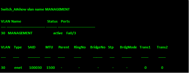
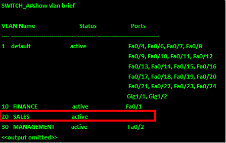
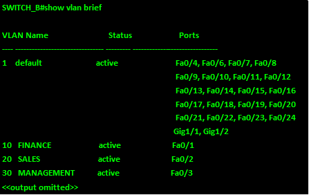
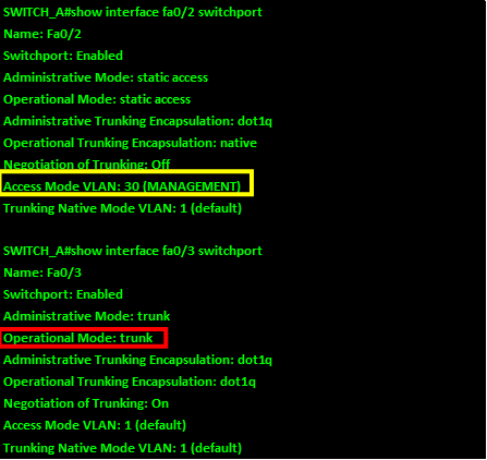
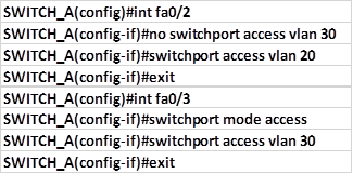
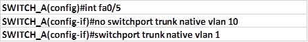
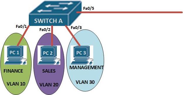
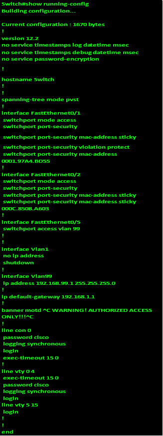
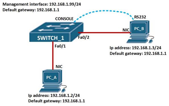
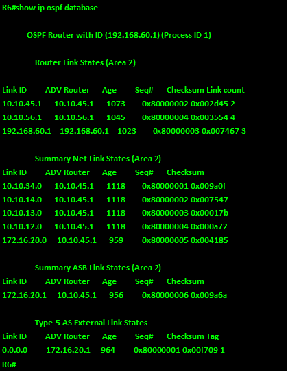
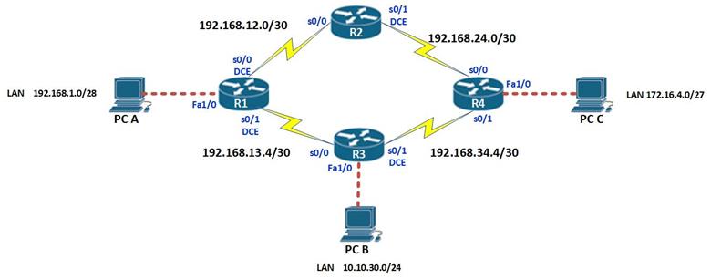
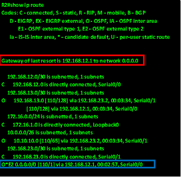
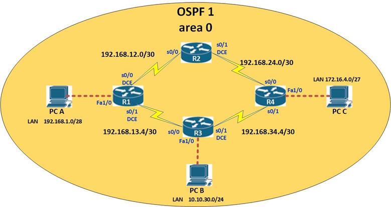
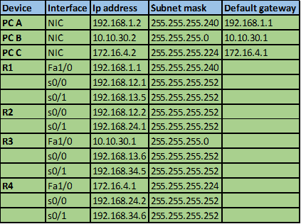
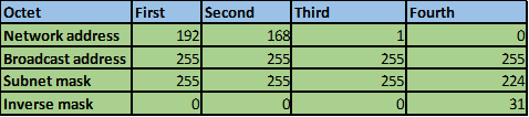
Author Archives: ccnablog

STP Part I

Overview

In the previous chapter, we looked at how we can segment a network using VLANs. In this chapter, we will discuss redundancy and how the end devices in the switched network are able to recover from a failure. We will discuss the role of STP in making sure that there are no loops as a result of redundant links in the network. In the second part, we will look at configuration of the various versions of STP and finally we will look at troubleshooting STP related issues.

All about redundancy

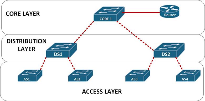
In earlier chapters on switching, we saw that the hierarchical network model is ideal in assignment of roles and functions in the network. We also saw that at the distribution and core layers of the network, redundancy can be achieved.

In the figure shown below, the access switches have redundant paths if the path on DS1 fails. Normally, users located on AS1 use the path shown in blue, however, if this path fails as shown by the red X, the frames would take the new path which is through DS2 as shown by the green arrow.

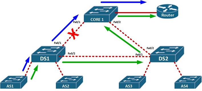
This is the essence of redundancy, to keep users connected even if there is a major failure on the network by taking an alternative path to the destination.

Layer 2 loops

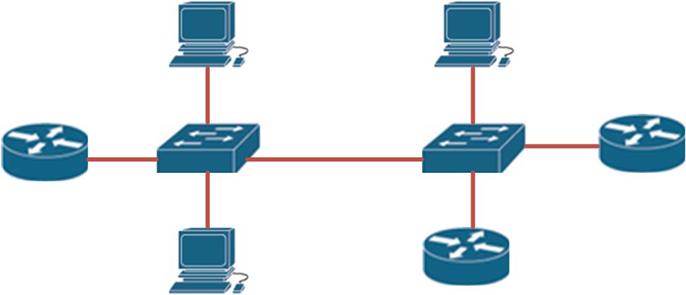
In as much as redundancy is a good thing in hierarchical switched networks, there is a very high possibility of loops. Take the scenario shown below.

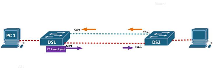
In this scenario, PC 1 wants to communicate with the node connected to DS2, the DS1 will receive the MAC address and the port for PC 1 and update its MAC table, it will then flood out this message out of all ports except the port it received the message on, which in this case is port fa0/1 and fa0/2. When DS2 receives the message, from fa0/1 first as shown by the purple arrow, it will update its MAC table with PC 1’s MAC and then broadcast the message out all ports except fa0/1 from which it received the message.

When DS 1 receives this message, it will “think” that PC 1 is directly connected to DS2 and thus it will update its MAC address table again.

The effect of this is that broadcast frames will go round the two switches, and since frames do not have the TTL field like packets, there will be a loop.

This can be a major disaster in a large network, and the loop may make the switch to behave like a HUB, since its MAC address table would eventually be filled up resulting in only broadcast traffic.

Broadcast Storms

The scenario shown above is a good example of a broadcast storm. It can be defined as a situation where there is so much broadcast traffic on a switch as a result of a layer 2 loop. This results in the consumption of all available bandwidth on the switch as eventually data cannot be forwarded by the switch.

Broadcast storms are caused by a loop in the network. A loop at layer 2 cannot be stopped since frames do not have a field that tells them that a frame has aged out. This is a major concern. We need backup paths in our LANs in case of failure and at the same time, we need to prevent loops.

Spanning Tree Protocol (STP)

Our networks need redundancy to protect the network in case a point fails, however, when redundancy is implemented, the likelihood of layer 2 loops increases. The spanning tree protocol, is a solution to the problem of loops in a switched network.

The Spanning Tree Protocol, works by blocking alternative paths to a networks and only allowing one path to be used. When the main path is disabled, STP reactivates the redundant paths and traffic continues to flow.

Consider the topology shown below:

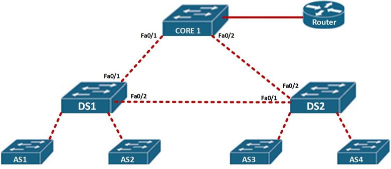
In this scenario, the path taken by AS1 and AS2, would be through fa0/1 to reach the router and fa0/2 to reach users connected to DS2. It would block the path between CORE 1 and DS2.

This would prevent a loop, if the link from DS 1 to Core 1 failed, STP on DS 1 would open up the blocked link – DS 2 to CORE 1, so as to recover from the erroneous link.

Spanning Tree Algorithm

The Spanning tree algorithm, is what STP uses to activate backup paths in the event of failure almost instantaneously. Similarly to algorithms used by routing protocols, the STA calculates the best paths in a LAN network and blocks alternative paths.

The root bridge

In a LAN network, Spanning Tree Algorithm elects a switch to be used as a central point in all the calculations, this is called the root bridge. This switch is ultimately responsible for the proper STP operation.

Root ports

The ports that are primarily used for forwarding frames in STP are the root ports. All the ports connecting to the root bridge on neighboring switches are root ports. When STP is fully converged, these ports will always be in forwarding state unless there is a failure.

Designated ports

The ports on the root bridges as well as one port on other links that are not directly connected to the root bridge are designated ports. In STP, these ports also forward frames.

Non – designated ports

When STP is fully converged, some ports will be blocked, these are the redundant ports. In STP, these ports are the non-designated ports and they can only become active in case of a failure.

In the topology shown below, all these ports are shown.

NOTE: there is always one designated port per link.

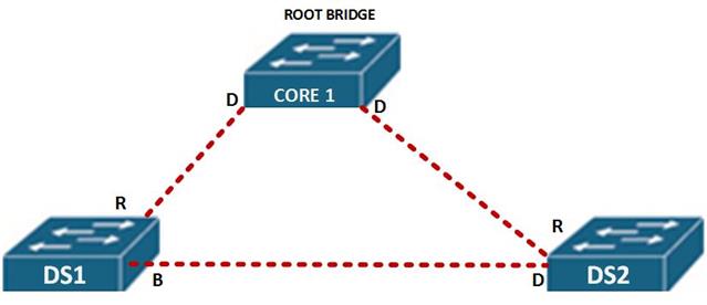
In this scenario, CORE 1, is the root bridge, therefore all its ports will be designated as shown by the letter D.

All the ports that lead to the root bridge, shown by R are root ports.

On the link between DS 1 and DS 2, there is one designated port and one blocked path. The blocked path is shown by B.

The reason that the port on DS 1 is blocked and not designated will be discussed later.

The root bridge

As mentioned before, the root bridge is the central point in STP and the main reference for calculations. The root bridge may be any switch on the network that wins an election process.

The root bridge election is determined by the BID (bridge ID). This field is made up of the switch’s MAC address and its priority.

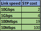
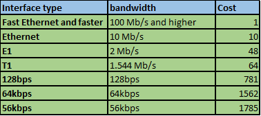
After the election of the root bridge, the STA will choose the best paths based on the bandwidth on the links or the cost. The costs of different speed links is shown below.

This field may be changed so as to influence the path that is made redundant.

NOTE: unlike in other protocols, where the higher the better when it comes to elections, e.g OSPF multi-access DR election, STP root bridge election prefers the lower values. Eg, lower mac address, lower priority, lower STP cost.

Election of the root bridge

In the previous section we said that the root bridge is used as the reference point for all STP calculation. The election of the root bridge is an important process and to understand STP, you must know it.

The BPDU (Bridge Protocol Data Unit) is a hello message, which is broadcast by the switches in the election process. The election process is illustrated using the topology below.

The BPDU, contains information shown below.

Root –ID: MAC address for the switch and its STP Priority

Bridge-ID: MAC address of the root bridge

Link cost – STP cost.

When the switches boot up, the BID and the ROOT ID is identical on each single switch in the network as shown below.

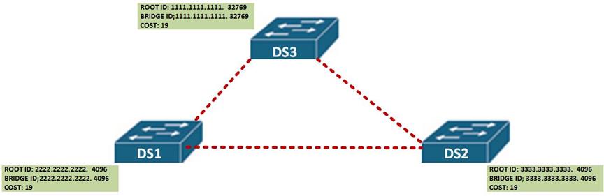
The switches then broadcast the BPDU frame with this information to the neighbors.

In our scenario, when the other switches receive the BPDU, they examine it against their own information to determine who the root bridge, in this scenario, when DS 2 and DS 3 receive this message from DS 1, they will identify DS 1 as the root bridge since it has a lower MAC address and priority of 4096.

When DS 1 receives this information, it will identify itself as the root bridge since it has the lower MAC address and priority.

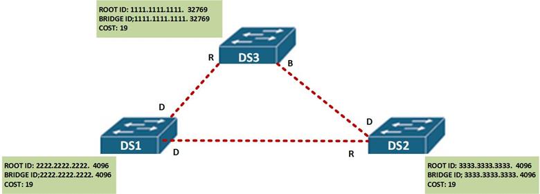
The STA will now determine all the ports leading to DS 1 on the neighbors as root ports and all the ports on DS 1 as designated ports.

The next step is to determine which port is blocked between DS 2 and DS 3.

In this case, the STA algorithm will look at which port between these two switches offers the lower BPDU, in this case, the port on DS 2 will be chosen and therefore will be marked as the designated. The port on DS3 will be blocked. The port roles after election are shown below.

STP states and timers

The determination of the spanning tree is based on the information attained as a result of exchange of BPDU frames between the switches. When the spanning tree is being determined, the ports on the switches transition from various states and use three timers.

These port states determine the status of a port as discussed below.

  1. Blocking state – any non-designated port or root port, is considered a port in blocking state. This means that any port that is not forwarding frames. This port state means that the port will only receive the BPDU frames so as to ascertain the location of the root bridge as well as to know when there is a topology change.
  2. Listening – in this state, STP usually knows that this port can send and receive frames, the ports in this state can send and receive BPDU frames to inform neighboring switches that it can be an active port in STP.
  3. Learning- in this state, a port is usually preparing to forward frames, the switch which has its ports in this state is usually populating its MAC address table.
  4. Forwarding – when the port is actively sending and receiving frames in the network, it is usually in this state. This port can also send and receive BPDU frames to determine if there are any topological changes.
  5. Disabled – when a port is in shutdown mode due to the configuration of an administrator, this is the state it assumes.

We will see the port states as we proceed in this chapter.

In STP, there are three timers that are used. These determine the state of the switch or port in the STP topology.

  • The Hello timer – by default transmitted every 2 seconds
  • The Forward delay – by default 15 seconds before transitioning to forwarding
  • Maximum age – by default 20 seconds

The hello timer is usually a message that determines if a link is still alive. The ports in the topology will receive a BPDU every 2 seconds. This is a keep-alive mechanism to determine if a port is still active in the STP topology. This value can be modified to a value ranging from 1 second to 10 seconds.

The forward delay is the duration that is spent by a switch in the listening state and the learning state, this value by default on CISCO switches is equivalent to 15 seconds for each state but an administrator can tune it to a value between 4 and 30 seconds.

The maximum length of time that a switch port can save the BPDU information is the max age time. This timer is usually 20 seconds but it can be changed to a value of between 6 and 40 seconds. When a switch port has not received BPDUs by the end of the maximum age, STP re-converges by finding an alternative path.

Portfast technology

On CISCO switches, some ports that may be connected to user nodes do not need to receive BPDUs and also need to transition immediately to the forwarding state. The CISCO portfast technology is a proprietary technology that allows such ports to transition immediately from blocking state to forwarding state.

STP convergence

To better understand STP, we need to understand the process a switch takes from boot-up to full convergence.

Step 1. Election of a root bridge.

Step 2. Election of the root ports.

Step 3. Elect designated and non-designated ports.

The election of the root bridge is through the sending of BPDUs, as we mentioned earlier, the switch with the lowest BID wins the election. The BID is made up of the SWITCH’s MAC address and the STP priority the switch that has the lowest BID wins the election and is made the root bridge.as we have mentioned earlier The root bridge is the reference or central point for all STA calculations.

The election of the root ports is the second step. The root ports as discussed earlier are the best paths to the root bridge. This is determined by the bandwidth available on each link.

The designated ports are non-root ports that can be used to forward traffic to the root bridge. There must be one designated port per link. All the ports on the root bridge are usually designated ports. Once they have been elected, STP chooses the links to block.

The ports that are blocked by STP are usually the ports that are not root ports or designated ports. These ports are marked as BLOCKED and will only be activated in case of a failure in one of the primary links.

STP process in action.

In this section, we will discuss this process by using the topology shown below, and finally we will determine Root Bridge and all the ports after convergence in STP using the information we have learnt thus far.

The topology shown below, shows the network topology which we will determine the STP ports and the root bridge for.

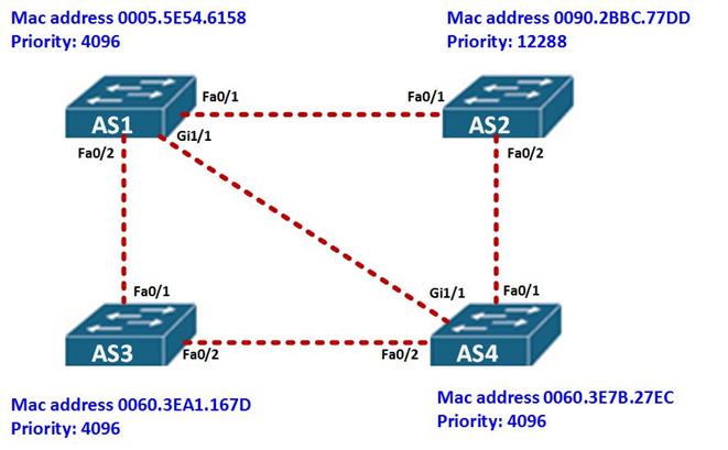
The first thing we need to determine is the root bridge. Based on the topology above, AS1 has a priority of 4096 and a mac address of 0005.5E54.6158, AS3 has a MAC address of 0060: 3EA1: 167D, while AS4 has a mac address and priority of 0060.3E7B.27EC, from this we can determine that the root ID of AS1 is lower since it has a lower MAC address, therefore it is the root bridge.

The other switches in this topology will add the Bridge ID value as the Root ID of AS1.

All the ports on AS1 will be designated while all ports on neighboring switches connected to AS1 will be root ports as shown in the diagram below.

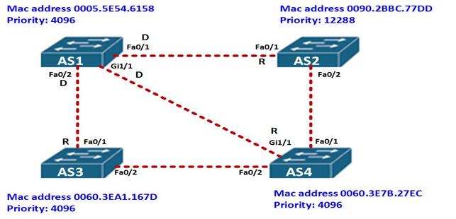
Next we need to determine which are the designated ports and the blocked ports on all the other remaining links.

From the topology above, the link between AS2 and AS4 is a FastEthernet link, however, the priority of fa0/2 on AS2 – 12288, is higher than that of fa0/1 on AS4 – 4096, therefore, fa0/2 on AS2 will be blocked and fa0/1 on AS4 will be designated.

The link between AS3 and AS4 is made up of FastEthernet links on both sides, however, the priority on both switches is the same, the tie breaker therefore will be the MAC address and in this case the MAC address of AS4 is lower. Therefore fa0/2 on AS3 will be blocked and fa0/2 on AS4 will be the designated ports. This is shown below.

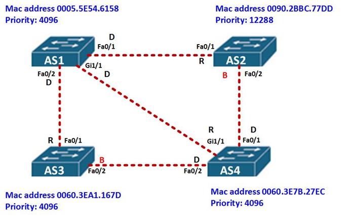
This completes the demonstration of the STP process on these switches.

Summary

In part 2 of this chapter, we will configure STP using the topology above, we will also incorporate the other concepts we have learnt in switching.
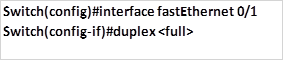
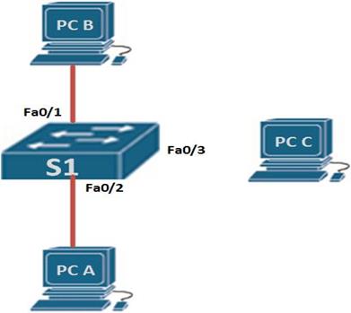
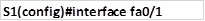
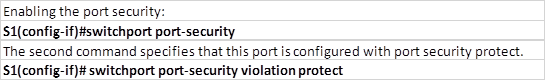
VLANs Part II

Overview

In part one of this chapter, we learnt how to configure VLANs on a switch. In this section, we will focus on deleting of VLANs on a switch, verification of configured VLANs as well as troubleshooting of some common VLAN problems.

Deleting VLANs

In other chapters, we have seen that using “no” at the beginning of a command is used to negate or delete configuration commands.

The configured VLANs unlike most of the commands in the IOS, are not stored in the startup configuration. If you issue the “show running-config” on switches, you will notice that the VLANs that were configured do not show up, this is because VLANs are not stored in the startup config rather, they are stored in a file known as: VLAN.dat.

To delete improperly configured VLANs, we use the command “no vlan <VLAN_ID>”, however, if we want to remove all the configured VLANs we issue the command “delete flash:vlan.dat ” in the privileged executive mode of a switch.

NOTE: you should be careful when using this command

Verify configuration of VLANs

To verify that the VLANs we had configured are in effect and operating in the proper ports, we use the command “show vlan brief” in the privileged exec mode on the switch. The output below shows the result of this command on SWITCH_A.

As you can see from the output above, there are eight VLANs on this switch. VLAN 1, 1003, 1004, and 1005 are usually on by default. VLANs 1003 – 1005 cannot be changed and they are reserved.

As you can see, the three VLANs we configured i.e VLAN 10 – FINANCE, VLAN 20- SALES and VLAN 30 MANAGEMENT, are all shown as active with the active ports indicated.

We can also use the command “show interface <interface_id> switchport”to verify the operational status as well as the configured VLAN on an interface. The use of this command on interface FastEthernet0/1 is shown in the output below.

From the output above, highlighted in blue; the switchport mode is shown as static access. This means that this port has been configured to operate in the access mode. The configured VLAN is shown as VLAN 10, further this port cannot negotiate a trunk link since the first line in the red box shows “negotiation of trunking is off.

The command “show vlan < name> <vlan_name>” or “show vlan <id> <vlan_ID>”, will show the specific VLAN and the ports that are configured in this VLAN.

NOTE: when you use the “name” option, the “vlan_name” keyword is case sensitive, this means it has to be exactly as the name configured for the VLAN.

The output of the command show vlan name <VLAN_Name> for the MANAGEMENT vlan is shown below.

As you can see from the output above, the vlan management has only 1 port which is fa0/3. The output of the command “show vlan id <VLAN_ID>” for VLAN 20 is shown below.

There are other commands such as the “show interface vlan <vlan_ID>” which are not discussed since they are beyond the scope of this course.

Troubleshooting common VLAN and trunking problems

In this section, we will troubleshoot some of the most common VLAN and trunk problems. To do this, the switches shown below have been configured and we will troubleshoot the problems with VLANs using show commands, after which we will fix them.

NOTE: to make this troubleshooting section more realistic, the configuration of the switches is not shown. Further, the end devices have been configured with correct ip addresses and default gateways as shown below, and to succeed in this lab, devices must be able to ping devices in their VLANs successfully.


The ip addressing for the end nodes is shown below.


Step 1: test connectivity

The first thing we will do is to test whether we can ping any of the nodes in the network. There are three VLANs with 2 PCs each, therefore we will ping each of the PCs in their respective VLANs to see whether there is connectivity.

The pings are:

PC 1 to PC 4

PC 2 to PC 5

PC 3 to PC 6.

All the fail, and from this we can deduce that there could be several problems.

  • Interface shutdown
  • Trunk misconfiguration
  • Incorrect switchport mode or VLAN assignment.

The “show VLAN brief” command on both switches should reveal which problem we are facing.

From the output of SWITCH_A above, we see that VLAN 20 has not been assigned port fa0/2, and VLAN 30 has been assigned port fa0/2 instead of port fa0/3. We therefore need to determine the operation modes of these ports and then fix the problems.

The “show interface <interface_ID> switchport” will show us the status of these ports.as shown below.

As you can see from the output of the “show interface fa0/2 switchport” and “show interface fa0/3 switchport” above, interface fa0/2 is configured to access VLAN 30 instead of 20 (highlighted in yellow) and interface fa0/3 is operating as a trunk instead of an access port (shown in red).

To fix this, we need to change the VLAN on fa0/2 from VLAN 30 to VLAN 20, we also need to change the operation mode of fa0/3 from trunk to access and assign it to VLAN 30. The commands shown below, are used to accomplish this.

This will fix the first problem. Attempting to ping is still not successful, therefore we need to check the trunk interface which in this case is fa0/5 on both switches to see whether there is any problem. To accomplish this, we issue the command: “show interface fa0/5 switchport” on both switches. The output is shown below.

As you can see from the output above, interface fa0/5 on switch_A is a trunk however, the interface fa0/5 on switch_B is in access mode. So we need to change this and see if communication will be successful.

The command needed on fa0/5 on SWITCH_B is:

this will change the operation mode from access to trunk, however, we still can’t ping successfully from PC 1 to PC 4, but pings from PC 2 to PC 5 and PC 3 to PC 6 are successful. Further, there is a message on the buffer as shown below:

The native mismatch problem, happens when the trunk links are configured with different native trunks.

NOTE: the native VLAN on switches should always be the same on a LINK. And it should not be a VLAN that has hosts assigned to it.

In this case, the native VLAN should be VLAN 1 not VLAN 10 as it is on fa0/5 on SWITCH_A. to correct this problem, we issue the following commands.

This should fix the error message and now there should be full connectivity between PC 1 and PC 4, PC 2 to PC 5 and PC 3 to PC 5.

Summary

The troubleshooting section of VLANs marks the end of this chapter, in this chapter, we’ve learnt about how we can segment broadcast domains on a switch using VLANs, effectively making smaller switches within the switch and each with its own subnet. We also configured VLANs and the trunk ports, we concluded by troubleshooting the various VLAN problems that may be encountered.

In the next chapter, we will look at the role of redundancy and loop prevention in our networks using STP.

VLANs Part I

Overview

In the previous chapter, we looked at the various concepts that make switches work. In this chapter, we will look at VLANs. We will discuss what they are, how they work and advantages of using VLANs in our LAN networks. We will also configure VLANs in our LAN networks.

What are VLANs

VLANs (Virtual LAN) are a way to divide the switch into different LAN segments. As we discussed earlier, networks connected to a switch are usually one 1 broadcast domain, this means that all devices that are connected to a switch use 1 IP subnet by default.

VLANs are a way in which we can divide the switch into smaller broadcast domains and therefore make it possible to implement many subnets on one switch.

A VLAN therefore, is a way to create multiple logical switches on a physical switch. Each logical switch uses its own IP subnet.

Consider the scenario shown below.

In this scenario, company XYZ has two departments; finance and sales. Each department has users located in both buildings at the same time each department is supposed to be on its own LAN segment, so as to separate the traffic between the FINANCE and SALES department. Typically, users on a switch are on 1 subnet which is a big problem. We therefore need a way to separate these departments which raises the question as to how to implement this solution. If a router is placed in between the buildings, we would require more than two Ethernet segments. And one switch would not be enough since these departments are on different subnets.

In this case, we can implement VLANs on a switch located between the two buildings. The users in each of the departments can then be assigned their own subnet.

This is one of the most significant uses of VLANs. As we continue with this chapter, we will elaborate on how VLANs are used in different scenarios depending on the challenges faced.

Why use VLANs.

The use of VLANs is very important in today’s networks. To appreciate VLANs, we need to consider why they are important.

  • Security – when we use VLANs, we can use one physical device for users with different access rights, the traffic in a sensitive group can use the same switch as that of a group with common traffic without violating the security policies.
  • Reduction of costs – by using VLANs, we can reduce the costs that would be needed if each department in an organization needed a physical switch. With a 24 port switch, and 20 users in different departments, we can implement VLANs to separate them without needing additional hardware.
  • Performance improvement – as we mentioned earlier, the default operation of a switch is in one broadcast domain. This means that if a frame is destined to a node that is not on the mac-address table, the switch has to broadcast it to all the ports. This can be degrade the performance of a network. With the use of VLANs on the other hand, the broadcast traffic is limited to a particular VLAN.
  • Administrative tasks improvement – the use of VLANs eases the work IT administrators have to perform to maintain the network. With VLANs, upgrading of the network, troubleshooting and other tasks are made easier. We will explore this in more detail as we progress.

Network without VLANS vs network with VLANs

In normal operation, when a switch receives a broadcast frame on one of its ports, it forwards the frame out all other ports on the switch. Take the scenario shown below.

If PC 1 wants to send a message to PC 6 on switch B, the frame would be broadcast to all the users connected to switch A and switch B. however, if we had VLANs as shown in the scenario below, the frames would only be broadcast on their respective VLAN.

The interconnection between the two switches is a trunk link meaning that traffic from many VLANs can pass through it. In the above scenario, traffic on any VLAN is limited to that VLAN only. Meaning that PC 1 and PC 2 cannot communicate and PC 2 and PC 6 cannot communicate since they are on different VLANs, however, PC 2 and PC 5 can communicate since they are on the same VLAN.

NOTE: VLANs divide the switch into logical groups on different subnets. The interconnection between two switches is usually a TRUNK port.

Trunks

When using VLANs on several switches, the interconnection the switches is usually a trunk. If we use an analogy of a highway, the trunk line can be likened to a highway which interconnects many small roads. The trunk link allows traffic from many VLANs to move between the switches.

The two types of trunk links that can be configured on CISCO switches are the ISL trunk and the IEEE 802.1Q trunk ports.

There are several concepts that you should know when it comes to configuring trunk ports, these are:

  • Native vlan
  • Dynamic trunk protocol

Native vlan

This is the port that the switch uses to send untagged traffic. Tagged traffic is all traffic destined to a particular VLAN. Untagged traffic may be any traffic which is not destined to any particular VLAN such as control information.

Dynamic trunk protocol

DTP is a CISCO proprietary protocol that negotiates the trunking modes between switches. As we mentioned earlier, the port between the two switches A and B, is a trunk port, therefore it carries traffic from all VLANs across the two switches.

There are three modes in which ports on a cisco switch can operate:

  1. Access
  2. Trunk
  3. Dynamic

An access port is a port that connects to an end device such as a computer or an IP phone.

A trunk port carries tagged and untagged traffic across switches and sometimes to a router.

DTP works by negotiating the operation mode of a port on CISCO switches. If one side is configured as a trunk, then DTP can determine the mode of operation on the other end of the connection.

These concepts and more will be discussed as we continue with the configuration of VLANs.

Configuration

In this section, we will configure VLANs based. The topology below consists of one switch and 3 nodes. Our task is to configure VLANs on this switch while keeping in mind that we might need to add another switch.

We will not configure the PC’s since we will not be testing communication between the PC’s.

In this topology, we are expected to configure the following:

  • Hostname of the switch
  • Console and telnet lines passwords
  • Switchports
  • Switchport security
  • VLANs
  • VLAN names

The first part which is the basic configuration is shown below.

Basic configuration

In the previous chapter, we learnt how to configure the switch’s basic operation. The commands shown below are a review of these concepts.

VLAN configuration

Part 2 is the configuration of the VLANs. In this scenario we have three VLANs i.e

To configure the VLANs go to the global configuration mode and type in the command:

the VLAN number is a unique number from 1 to 1005, however there are reserved VLANs which we will discuss later.

After executing this command, we will be taken into the VLAN configuration mode denoted by prompt:

in this mode we can name the VLAN as we have been instructed. In our scenario, the configuration commands needed to configure all the three VLANs are shown below.

Assign ports to the VLANs

Next we need to assign the ports on the switch to the VLANs we have configured. To do this we need to enter the interface configuration mode and follow the steps shown below.

For PC 1 which is connected to fa0/1

The command: switchport mode <access> specifies that this port is an access port and therefore it can only support traffic from 1 VLAN.

The second command: switchport <access> <vlan 10> specifies that the node connected to this port can only access VLAN 10, therefore the ip subnet for this port should be the same for all nodes on VLAN 10.

The commands needed to assign the switchports connected to the three PCs to their VLANs are shown below.

Configure port security

Now that we have assigned the ports to their respective VLANs, we need to configure port security for the three ports.

All three host ports, will use dynamically learnt mac-addresses, we will use a maximum of one MAC address per port, and configure the violation mode as shutdown. These commands are shown below.

Configure the trunk port

The last thing we will configure will be the trunk port which in our case is fa0/5

To configure this port as a trunk port the commands needed are:

The command: switchport trunk native vlan 1, specifies that the native VLAN on this switch is VLAN 1.

NOTE: it is advisable to configure the native VLAN using an ID other than the default which is VLAN 1 for security purposes.

Summary

This is the last configuration command we use in this scenario. In part 2 of this chapter, we will learn how to verify VLANs operation, delete VLANs and troubleshoot common VLAN problems such as native VLAN mismatches.

Switch Concepts and Configuration Part II

Overview

In the previous part, we looked at some of the concepts behind switch operation. In this chapter, we will continue with the configuration and verification of the basic switch configuration, configure and verify port security on a switch and learn some other important concepts.

Duplex settings

As we mentioned in part 1 of this chapter, the duplex mode determines whether communication will be unidirectional or bidirectional. By defaults, the duplex on CISCO switches is usually auto. This means that if one side is operating on half-duplex, then the port would be in half-duplex as well.

We can hard code the ports on the switch to use only full duplex since it is the preferred mode. The commands needed are implemented in the interface configuration mode on a switch as shown below.

Port security

There are several security breaches that switches are vulnerable to. In this course however, you are only expected to understand some basic security options such as port security.

There are several attacks that switches are vulnerable to such as:

MAC address flooding – in this type of attack, an attacker usually gains access to a switch using a node. They then use a tool to send invalid source MAC addresses to the switch. Switch operation works by adding the MAC address to the mac-address-table which is limited to a certain number of MAC-addresses. When this database is filled up, the switch is unable to forward traffic using unicast and it begins to operate like a hub by flooding frames out of the ports. This means that the attacker can see all the frames for the nodes in the network.

MAC-address spoofing – in this attack, an attacker poses as a DHCP server, when legitimate clients request for addresses from the DHCP server, the attacker responds with an address that would permit them to see the traffic from a particular node.

Other common attacks may be aimed at CDP, telnet or other technology weaknesses that may be manipulated through the switch.

Using port security is one way to protect the switch against such attacks. All switch ports or interfaces should be secured before the switch is deployed. Port security limits the number of valid MAC addresses allowed on a port.

Secure MAC Address Types

Port security is one way of securing a CISCO switch. Configuration options using port security can secure the switch in the following ways.

  1. Use of statically configured MAC addresses: this entails assigning each port on a switch to a particular user node by hardcoding the user’s MAC address to the port. This means that only devices matching the configured MAC addresses can communicate. This is a good way to implement security, however, it may be an administrative nightmare to configure the MAC addresses of the clients to the switch due to the size of the network.
  2. Using dynamic secure MAC addresses is a good way to ensure security on a switch. The switch ports are configured to learn and store the MAC addresses of the user nodes.
  3. Using sticky MAC addresses is a good way to ensure that only dynamically learnt MAC addresses can use the switch, these addresses are then saved to the running configuration file of the switch which means that they are lost when the switch is rebooted.
  4. We can also specify the maximum number of MAC addresses that can access a particular port. This is a good way to secure against MAC address spoofing.


In this case we will be using a modified topology to configure port security. The topology shown below consists of 1 switch and three host nodes. PC A, PC B and PC C. we have connected only PC A and PC B to the switch and we will use PC C as the test for security.

When configuring port security, there are several Security Violation Modes that are used to protect the switchports.

Security violations

The security violations determine the action to be taken if access on a port does not meet certain criteria.

The violations apply when the maximum number of user nodes that can access a port is reached, when a particular MAC address that has not been learnt dynamically or statically tries to access the switch or other criteria that may be configured according to the security policies in place in an organization.

The violations that can be triggered due to these events include:

  1. Protect – in this mode, the switch will drop the frames from a node that breaches security, however, it will not inform the administrator of the security breach.
  2. Restrict – in this mode, if a violation of the security policies is made, the port drops the frames from that port and records the breach. In most cases, this entails sending an SNMP trap, increasing a violation counter, and sending a syslog message.
  3. Shutdown – when a violation is detected, the port that the frames were received on is shut down. The switch also sends a message to the administrator using s SNMP and syslog. The violation counter also records the breach. In this mode, the administrator is the only one who can re-activate the port after investigating the breach.

In our scenario, we will configure port connected to PC A as security violation restrict, the port connected to PC B will be in violation mode restrict and port Fa0/3 will be in violation mode shutdown.

To configure the secure ports as we have mentioned above, follow the steps shown below.

Step 1.Configuring port security protect on port fa0/1.Enter the configuration mode for interface fa0/1


Step 2: in the interface mode, enter the following commands to activate port security and then enable the protect violation mode:


Step 3. We need to bind the mac address of PC A to port fa0/1 such that if another node is connected to this port, the interface will deny this port from transmitting. To do this, we will configure the port with a static mac address of PC A. as shown below.

The mac address keyword is the configured mac address on the PC’s NIC.    

Step 4: is the final step is to specify the number of MAC addresses that can access this port. In our case we will specify only one so that if any other device tries to access this port, the port will be protected.


In our case we use 1.

After this configuration, save the configuration to the NVRAM.

To configure port security violation restrict and shutdown, the commands are shown below.


We can also configure the type of mac addresses we would like to access a specific port. Using the static mac address is good but can be tedious in a network with thousands of mac addresses.

In this case we use sticky mac addresses, this means that when a node is connected on a switchport, it’s mac address is learnt and stored in the switch’s memory. To configure sticky mac addresses we use the command:

It is recommended that you should also configure the maximum number of mac addresses on a port so that no one can use other devices such as hubs.

Now that we have configured port security on the two ports, we need to verify their operation.

On port fa0/1, we have configured the port for violation mode protect and on port fa0/2 we have used the violation mode shutdown. Both ports are configured with nodes.

The command show port-security <int type and number>, shows the protection status on a port. The output of this command for port fa0/2 is shown below.

As you can see from the output above the port security is enabled and the port is shown as secure. The violation status is shutdown and there is one sticky mac address that has been learnt by this interface.

To see whether this security will work, we will connect PC_C to this interface and view the output of this command. The output is shown below.

As you can see from the output above, the violation count moved from 0 to 1 and the port status is shown as “secure-shutdown” meaning that it has been deactivated till an administrator intervenes.

With this configuration, we have finished the security configuration options that we need to configure on our switches. In the next section, we will look at the various verification and troubleshooting commands that you need to know when configuring a switch.

Verification and troubleshooting commands

There are several commands that can be used to verify the operation of a switch as well as to troubleshoot when there is a problem. Some of these commands we will discuss later as we continue with switching but some of the basic ones are shown below.

Show running-config

Just like on routers this command will show the configuration that is currently in use on the switch. The output of this command on S1 is shown below.

With this command, you can be able to view most of the configuration options that have been made on the switch. This command can be useful when verifying whether the configuration commands that were used are correct.

Show mac-address-table

This command will show all the mac addresses that the switch knows about. It can be useful when you want to verify whether the switchports have nodes on them. Since we have configured only 2 ports on our switch, the mac address table will only have 1 entry with the mac addresses of the two PCA since the port attached to PC 3 as we configured was shutdown due to a violation, this is as shown below.

Show interface <name and number> switchport

This command will show various statistics for the switchport. More of this will be discussed in later chapters.

Summary

In this chapter, we have looked at the various configuration options for security on switch ports, we have also looked at various verification commands. In the next chapter, we will look at VLANS. This chapter is supposed to introduce you to the concepts behind switch operation, as well as basic switch configuration.

The concepts in this chapter are an integral part of the ICND 1, ICND 2 and CCNA composite exams. In the next chapter, we will look at a topic that is at the heart of switch operation which is VLANs.

Switch Concepts and Configuration Part I

Overview

In this chapter, we will explore switching concepts and the basic configuration of a switch. We will discuss the switch’s operation, layer 2 and layer 3 switching as well as other concepts. We will conclude with the basic configuration of a switch and this will lead us into the discussion on VLANs.

CSMA/CD

We discussed the CSMA/CD in the chapter on Ethernet, we said that the LAN networks operate using several rules. In this type of communications, devices on the same Ethernet segment usually listen to the network media to determine if they can transmit or whether they have to wait. With hubs, only one device could transmit at a time, however, with switches, multiple devices can use the media at the same time.

Ethernet communication

In Ethernet communication, we have three types of ways in which messages are transmitted.

  • Unicast
  • Multicast
  • Broadcast

Unicast

With unicast communication, a frame is usually sent from one node to a specific destination. In this mode, there is only one sender and one recipient. This means that the sender and the recipient as well as the switch in the middle must know about one another. In modern LANs, this is the most common form of communication especially on the internet using protocols such as HTTP, Telnet and others.

Multicast

In multicast communication, the sender usually transmits a frame to a group of nodes on the Ethernet segment. The type of protocol in use can typically determine whether multicast is used. In a teleconferencing call for example, a user may need to communicate with three other users simultaneously. In this case, multicast messages will be sent.

Broadcast

In case a user node needs certain information and it does not know who has the specific information, it may use broadcast type of communication. In this case, a frame is usually sent to all the devices on the same LAN. This communication is also useful if the message being communicated is meant for a large audience.

Addressing

In the Ethernet, the type of addressing used is the physical address which is typically the MAC address. This is the address that is used to communicate frames. When packets are received from the network layer, they are encapsulated into frames. This includes adding information such as the source and destination MAC address.

MAC address

As we have mentioned, the MAC address is the address that is used in the Ethernet. The address itself is made up of 48 bits which are represented in hexadecimal numbers.

When we were looking at layer 3 addressing, we said that IP address consist of two parts, the network and the host segment, similarly the MAC address is also broken up into two parts.

  • the Organizational Unique Identifier (OUI)
  • the vendor assigned number

The OUI consists of the first 24 bits of the MAC address. It is usually the code that has been assigned by the IEEE to a particular vendor. In CISCO switches for example, the OUI is usually: 0009.7C

The next 24 bits are usually a number that is assigned by the vendor for that particular device. It uniquely identifies the device hardware.

The entire MAC address is usually hard coded to the hardware of the switch and cannot change.

Duplex settings in Ethernet

On Ethernet networks, there are two modes of operation; the duplex determines whether the communication is unidirectional or bidirectional. The two duplex modes are:

  • Half duplex
  • Full duplex

Half duplex

In this type of communication, transmission of data is only one way, this means a device can either send or receive frames and not both. When HUBs were common in networks this was the communication that was used. This type of communication can be likened to using a walkie-talkie where you can either talk or listen but not both. While using the half duplex communication, the likelihood of collisions is high, therefore, CSCMA/CD is used to minimize them.

Full duplex

Full duplex communication provides for bidirectional flow of data. This means that devices using this type of mode, can send and receive frames at the same time. In modern switches, this is usually the default mode of operation. The chances for collisions are minimal.

The mac address table

When we were discussing the operation of routers, we said that the forwarding decisions routers make are based on the information in the routing table. Similarly, the switches also have a database that contains addresses. This database is called the MAC-Address table and it is the basis by which switches forward frames.

When communicating, the switch uses this database to determine the source and destination of frames.

The steps taken when a switch wants to forward a frame are shown below.

  1. The frame is received by the switch from a port.
  2. The switch checks whether it has the source port from which it received the frame. If it does not it adds the source MAC address to its MAC address table.
  3. The switch then checks whether it has the destination port for the frame in its MAC address table, if it does not, it broadcasts the frame to all the ports except the port it received the frame on.
  4. When the destination node replies, the switch adds the MAC address to the MAC-address table and subsequent communication to this node will be unicast not broadcast.

The figure below shows an example of the mac-address table.

Configuring the switch

We have learnt of the IOS configuration modes as well as the basic configuration in a previous chapter. We saw the different modes as the user executive mode, the privileged executive mode, the global configuration mode and various specific configuration modes such as the interface configuration. In this section, we will configure some of the basic options in a switch which include:

  • Hostnames
  • Banners and passwords
  • Management ip address
  • Duplex settings
  • Console lines and vty lines.
  • Duplex settings

In the second part of this chapter, we will look at other switch concepts and configure other options as well as verify the switch’s operation.

The topology we will be using for this configuration is shown below.

In this topology, we have 1 switch and 2 hosts. We will configure the switch using the console cable. Create this topology in packet tracer or a physical lab and follow the steps shown:

Hostnames, console & vty lines, banners and passwords

On more modern switches such as the CISCO 2960 switch which is the one we are using, the CISCO IOS is used, this is unlike older switches such as the catalyst switches. Therefore, most of the configuration commands we will use are similar to those used when we were configuring routers.

On SWITCH_1 command line interface, we need to enter the global configuration mode so as to configure most of the options. To access this, enter the following commands.

The first command gives access to the privileged access mode while the second, which is “configure terminal” will give us access to the global configuration mode.

In the global configuration mode we need to first change the hostname of the switch from “switch” to “SWITCH_1“. To do this, we enter the command: hostname <SWITCH_HOSTNAME>

In our scenario, this command is shown below.

When this command is executed, the prompt will change from “switch(config)#” to “SWITCH_1(config)#“.

Next we need to configure the line console and the 5 telnet line options such as the password, executive timeouts, and logging synchronous. The commands shown below are used to configure the passwords on both lines as “cisco” and the timeouts as 15minutes.

The command logging synchronous will prevent unnecessary messages from appearing on the screen while typing and thus disrupting the command while being typed.

The banner is a message displayed when someone tries to access the switch, with a message. We discussed some of the reasons that may make an administrator want to use a banner. In our case, we will use a banner MOTD which is configured using the command:

The pound symbol is used to indicate the beginning and end of the message. In our case we will use the message “WARNING. AUTHORIZED ACCESS ONLY!!!” which is configured using the command shown below on SWITCH_1.

When we were configuring routers, we noticed that to access the router remotely using the vty lines, we used an ip address. In switches, we need to configure an ip address, subnet mask and a default gateway much like a PC, the ip address is used to manage the switch.

By default, CISCO switches use VLAN 1 as the management VLAN, but it is advisable to change this since this can be a security vulnerability.

To enable management of the switch via a management interface, we need to create a management VLAN and assign it a management ip address. In our case we will use the VLAN 99 and issue it with an ip address of 192.168.99.1, this will allow the switch to be managed remotely via telnet lines.

We also need to configure default gateway so that traffic to remote networks can be accessed via the switch.

In our scenario, the default gateway will be 192.168.1.1

To configure the management interface, we follow the steps shown below.

NOTE: the “interface vlan command” is used to configure an SVI (switched virtual interface)

Step 1. Create the management VLAN interface, which is VLAN 99. Creation of VLANS will be discussed in more detail in the next chapter. However, the command we will use in this case is:


Step 2. Assign the interface with an ip address and subnet mask and activate and make it operational using the no shutdown command.


Step 3. On one of the switch interfaces, we need to link it to VLAN 99 management vlan, this is done as shown below. These concepts and commands will be discussed in part 2 of this chapter and also the chapter on VLANs.

To configure the ip default gateway so that traffic destined to remote networks can be forwarded we use the command “ip default-gateway <ip address>” command. In this scenario, the ip address we will use as the default gateway is 192.168.1.1 and this command is implemented as shown below.

After this configuration, all the devices on the network should be able to communicate without any additional configuration.

As you can see from the statistics of PC_A below, pings to PC_B are successful.

Summary

In part 2 of this chapter, we will look at a few more concepts on switching and configure more options such as port security, we will also take a look at the various verification and troubleshooting commands that can be used on switches.

Introduction to LAN switching

Welcome to the world of LANS, in the previous couple of chapters, we learnt about routers and how they are used in the networking environments. In the next couple of chapters, we will learn about LANs and the main device we will use will be the SWITCH. The concepts we will learn will also tie in with routing concepts.

LAN DESIGN

Overview

In today’s business environment, businesses need information to survive. With technology, this has been made possible, the use of new methods of communicating such as the use of voice, video, data which is transmitted over networks is crucial. As such, we need to design LANs with these needs in mind. In this chapter, we will discuss some of the considerations to make while we design the LAN. We will look at the hierarchical LAN model and its benefits, some design considerations as well as the benefits of well-designed LANs. This chapter is meant to introduce you to the world of LANs.

LAN design concepts

CISCO not only designs and produces network equipment, but also they focus on developing the most optimal way to use their devices, as such when designing a LAN network, they recommend that a hierarchical model. In this type of architecture, there are a few things that have to be observed:

  • Network segmentation and broadcast traffic management – this is mainly through the use of VLANs
  • Security
  • Easy configuration and management of the switches
  • Redundancy

These concepts will be explored in more detail as we explore LAN design.

Hierarchical layered model in LAN design

As mentioned earlier, the design of a LAN network is critical to communication within the enterprise, when using the hierarchical model as recommended by CISCO, there are three layers that we should implement depending on the size of the organization.

  • Core layer
  • Distribution layer
  • Access layer.

The figure below shows how the implementation of this hierarchy can be achieved.

Starting from the bottom, we have the access layer. This is the layer that connects to end user devices such as PCs, printers, IP phones among others.

The distribution layer, is meant to aggregate the data from the access layer. This layer controls the traffic in the lower levels and prioritizes traffic based on organizational policies that have been implemented during configuration of the switches. Typically, this level should be redundant and made up of faster switches than the access layer.

The core layer, is responsible for high-speed switching in the network. Typically, this layer should consist of the fastest switches in the network and offer the highest bandwidth since communication to other networks from the lower levels is forwarded through these switches.

Benefits of a hierarchical model

  • Scalability – when you implement a network a hierarchical network model, expansion is simplified since all the roles are well defined. For example, if you have 5 access layer switches, connected to 2 distribution layer switches, you can add the access layer switches until all the ports on the distribution switches are filled up.
  • Redundancy – this is achieved when the switches in each layer are connected to two or more devices at another level. If one device at the higher level in the hierarchy fails, the lower level switch automatically fails over to the other switch. Redundancy is achieved at the distribution and core layers.
  • Performance – it is recommended that core layer switches should have very fast switching abilities. The distribution switches should also be very fast and redundant. The result of using very fast core and distribution layer switches would guarantee very fast networks.
  • Security – the security of the network is enhanced since at each layer of the model, there are several security measures that can be put in place; for example switch ports at the access layer can be configured with port security, segmentation of the distribution layer using VLANs is also another security feature.
  • Manageability is the ability to make configuration changes in the network, the use of the hierarchical model eases management of the switches. For example, making changes on one layer would be simplified since we can assume that the role of switches in that layer all perform similar functions, further, the modular design means that management does not mean that the network is down due to maintenance due to redundancy.

Considerations when choosing a switch

  • When deciding the switch we should implement for our LANs, there are several considerations that we need to take in mind. These might be influenced by the organizational policies while others might be influenced by the technological needs.
  • Switches with fixed configurations are switches that cannot be modified by adding additional modules, these are lower level switches and are ideal for the access layer functions.
  • For more flexibility, we might need modular switches, these switches typically allow us to install modules such as more switching ports, these would be ideal for rapidly expanding networks that need to be changed frequently.
  • To provide high bandwidth, we may need to interconnect special types of switches which have a stackable ability using a backplane cable. These would be ideal for high bandwidth requirements in a large network at the core layer.
  • Port density – this is the number of ports on a switch. In many cases you will find switches with 24 or 48 port switches. This can be a design consideration since you may need to consider the inter-switch connections.
  • Forwarding rates are the processing capabilities of the switch. The forwarding rate is measured by calculating how much data the switch can process in a second. This is different from the bandwidth that is available on its ports.
  • In most modern networks, the use of IP phones is prevalent, most of these devices get power over the LAN interfaces connected to switches using a technology called POE (Power over Ethernet). As such, when deciding which devices to buy, PoE should be a feature that should not be overlooked.
  • In recent times, switch designs have been changed so as to support layer 3 functionality, as you may already know, switches work at layer 2 of the OSI model, however, implementing layer 3 switches gives more options such as routing, IP addressing and other options.

Access layer switch features

There are several features that a switch at each level of the hierarchical model should have. As we mentioned earlier, the access layer is the lowest level in the hierarchical LAN architecture, at this level user devices gain access to the network over a number of devices. As such, the features at this level include: VLAN support on the switches, Fast Ethernet and Gigabit Ethernet links, PoE and support for link aggregation so as to increase the switching speed.

Security is important in our networks, at this layer, we can implemnent several security measures such as port security to control access to the network.

CISCO recommends that VLANs be localized to a switch, the switches at this level should have support for VLANs for a variety of purposes.

Link aggregation is the ability to use multiple links at the same time. This is a more effective way to use the bandwidth available on the switches.

To support multiple devices on a single port, PoE is an important feature, it allows us to use the switch to power certain devices in our network such as IP phones and Wireless controllers.

The ports on access layer switches should be fast enough to support the evolving bandwidth needs of the enterprise. As such, Fast Ethernet which offer speeds of up to 100Mbps and Gigabit Ethernet links which offer speeds of up to 1Gbps should be used.

Distribution layer features

At the distribution layer, communication across the various access layer switches should be supported, this means that these switches should offer more features than the access layer switches. Features such as redundancy, faster ports than the access layer, layer 3 support should be implemented at this layer.

  • The use of security policies is a security feature that should be implemented at the distribution layer, some of these may include the use of access lists.
  • Inter-vlan routing which is making communication between different VLANs possible should be available at this layer.
  • The ports at this layer should be very fast, typically, Gigabit Ethernet and 10 gigabit Ethernet links should be used. These ports should be aggregated and redundancy should be implemented between the switches.
  • At this layer, we need to prioritize the traffic from our access layer, as such, QOS (Quality of Service) mechanisms should be implemented.

NOTE: at the distribution layer, the use of layer 3 capable switches is highly recommended so as to support most of the features mentioned above.

Core layer features

The core layer of the network is the main link between our internetwork and other networks such as external networks. At this layer of the hierarchical model, there should be very fast switching, security policies, redundancy, layer 3 functionality and quality of service. In some organizations, the core layer may not be needed if the network is small.

  • At the core layer, we should have very fast switches, typically operating at 10 gigabit speeds and above. This is to support the requirements of all the access and distribution layer switches.
  • At this level, the use of security policies to control access should be implemented. This means that the switches at this layer should have layer 3 support.
  • The core layer is sometimes implemented as the gateway to external networks and therefore redundancy is also an important element.

In the forthcoming chapters, we will discuss some of these concepts in detail through the networks that we will design and implement. The concepts in this chapter are meant to give you a firm foundation on the LAN architecture as recommended by CISCO. For more on this, you should conduct more research to discover best practices when it comes to designing and implementing LAN networks.

Summary

In this chapter, we have introduced the LAN. We have looked at the hierarchical layered model when designing LANs. In the next chapter, we will discuss switch concepts and the basic configuration of a switch.

OSPF Part IV

Overview

In part 1 and part 2 of this chapter, we looked at the basic configuration of OSPF and further learnt more OSPF concepts such as redistributing the static routes and the metric, in part three, we looked at multi-area OSPF. In part four, we will look at OSPF and multi-access networks, we will conclude with a more complex OSPF lab which will be vital not only in the ICND 1, ICND 2 and CCNA composite exams but also in real world scenarios.

Multi-access networks

Multi-access networks, are networks that consist of more than 2 devices sharing the same media. In the example shown below, the three routers and three PCs are interconnected using the two switches at the center of the topology. This means that the interfaces on the routers that connect to the switches as well as the PCs are in the same subnet.


On the other hand, in Point-to-point networks, there are only two devices on one subnet. The figure shown below shows two routers which are interconnected using a WAN link. This is an example of a point-to-point network.

In OSPF, we can have 5 network types which are:

  • Point-to-point
  • Point-to-multipoint
  • Broadcast Multiaccess
  • Virtual links
  • Nonbroadcast Multiaccess (NBMA)

In the CCNA course we focus on the OSPF point-to-point networks and broadcast multi-access networks. The other network types are discussed in more advanced courses such as CCNP and CCIE.

Challenges in OSPF Broadcast multi-access networks

In broadcast multi-access networks, we are faced by two challenges in an OSPF environment.

  • Multiple adjacencies
  • Flooding of LSAs

Multiple Adjacencies

As we discussed earlier, neighboring routers in OSPF usually create adjacencies with each other. In broadcast multi-access networks, this is a major issue.

Consider the network topology shown below. In point-to-point networks, we were used to neighbors being directly connected routers, in the example shown below, the four routers are all directly connected because they are in the same subnet.

This means that the routers in this example would flood LSAs between each other and create adjacencies with one another.

To get how many adjacencies would be created, the formula shown below can be used:

n (n-1)/2 where n Is the number of routers.

In the scenario below, we have 4 routers, using this formula:

n(n-1)/2 we get: 4(4-1)/2 = 6

This is shown in the scenario below and the adjacencies are highlighted by the blue arrows.

The number of adjacencies in this scenario are few, but can you imagine a large network such as one with 100 routers. This can be problematic and a big burden on the routers’ resources.

Flooding of LSAs

As we have learnt previously, OSPF uses triggered updates which are flooded to all concerned routers. Take the scenario above, if R1 lost a route to its LAN interface, this information would be broadcast to R2, R3 and R4, these routers would in turn flood that information to every router in the network except where the information originated from causing a routing loop. This is demonstrated in the figure below.

The green arrow shows the network that is down on R1. As you can see this information is propagated to R2, R3, and R4 several times which can cause a routing loop.

Solutions to OSPF broadcast multi-access problems

In OSPF, these challenges are solved by electing the DR (designated Router and the BDR (Backup Designated Router).

In the first instance, we saw that when a network on R1 went down, all the routers were flooded with updates about this missing route. However, with the election of the DR as shown above, R1 only informs the DR router – R2, about the missing route. The DR then updates the other routers in the multi-access network.

NOTE: in our scenario above, we have not included the BDR, however the BDR is also informed of the missing route, but it does not update other routers unless the DR is down in which case it is elevated to the role of the DR.

The election of the DR and the BDR in OSPF is a very important factor and it stops the problems we have seen. When the DR and BDR are elected, all other routers in the multi-access network become DROther, this means that they are neither the DR nor the BDR. The DROther routers will never update other routers in the network.

Election of DR and BDR

How do the DR and BDR get elected? The following criteria is applied:

  • First. elect the router with the router that has the highest OSPF priority as the DR
  • Second. Elect the router with the second highest OSPF priority as the BDR
  • Third. If the priorities are equal, the DR is elected based on the highest router ID.

In the previous section, we discussed that the router ID is selected based on the following criteria.

  1. Router ID as configured using the router-id command
  2. Highest loopback interface
  3. Highest active interface in the OSPF domain.

Based on the information above, we can determine the DR and the BDR in the topology below.

Based on the topology above, two routers are candidates for the DR, R2 and R3 this is because they have the highest router priority in the network. However, R2 has a higher router ID and therefore it will become the DR, R3 will become the BDR and will be used ONLY if R2 fails.

Promoting the BDR to the DR

The DR never changes unless one of the following happens:

  • The DR fails.
  • The interface connected to the multi-access network on the DR goes down.
  • The OSPF process on the DR goes down.

If one of these situation happens, the BDR router is automatically elevated to the role of the DR. the routers then conduct an election to determine the new BDR. If the previously failed DR comes back online, it does not resume its role as the DR, rather, it assumes the role of a DROther.

Router priority

In most cases we would like the DR router to be selected through preference. In this case, relying on the router-ID may not be enough. The router priority in OSPF, is used to determine which router becomes the DR and the BDR in the Ethernet section as mentioned earlier.

Changing the router’s OSPF priority is key in ensuring that the right router is chosen as the DR.

To configure the router’s priority, we use the command “ip ospf priority <0- 255>” in the interface of a router which is participating in OSPF.

NOTE: A priority of 0 means that the specified router will never be the DR.

Now that we know of the concepts in OSPF and multi-access networks, we will now do a lab on these concepts and get to see how they work.

OSPF Topology

The figure shown below shows the topology we will be configuring. As you can see we have 6 routers which are all connected to 1 switch. They are all in 1 Ethernet segment in the 192.168.1.0/24 network.

Each router in this topology is using an ip address that corresponds to its router number.

In this scenario, we are supposed to configure OSPF on all the routers and at the end of the chapter, we should be able to determine which routers will be elected as the DR and the BDR.

R1, R3, R4 and R6 all have loopback interfaces with the ip addresses shown in the diagram.

NOTE: after configuring the fast Ethernet interfaces that connect to the switch leave them in shutdown mode.

The router ID’s and ospf priorities in use are shown in the table below.

In our scenario, the basic configuration of the router has been done; our task is to configure OSPF and to determine who will be elected the DR and the BDR.

Configure OSPF

The first thing we need to configure in this scenario is OSPF on all routers. This means using the network command.

In our case we are using OSPF process id of 1 and area 0.

The table below shows the OSPF configuration statements on each of the 6 routers.

As you can see from above, all the network statements have been configured, but no routes will be advertised since the interfaces connecting the routers to the switch are in shutdown mode.

Configure OSFP priorities

The next step is to configure the OSPF priorities, this is done in the specific interface that is connected to the multi-access device using the command:

In our scenario, all routers have the same interface that is connecting to the switch which is FastEthernet 0/0.

Therefore, in each of these interfaces we will configure the OSPF priority as shown above:

The configuration of R1 and R4 is shown below.

After configuring the OSPF priority on all the routers, enable the interfaces which connect to the switch by entering the “no shutdown command”, this should enable OSPF to learn of the routes in the network.

The output of the “show ip route” command on R1 is shown below.

As you can see, R1 has learnt of all the routes from the neighbors.

To confirm which router is acting as the DR, we use the “show ip ospf neighbor” command on each of the routers. The output of this command on R4 is shown below.

As you can see from the output, R4 has formed full neighbor relationships with all the routers in the network, further, since neighbor 1.1.1.1 is marked as the BDR and all the other routers as DROTHER, this router is the DR for this network.

The output of the “show
ip ospf neighbor” on R3 should show who the DR router is.

NOTE: neighbor 4.4.4.4 is in the state of “FULL/DR” and neighbor 1.1.1.1 is in the state of “FULL/BDR”, the other routers are listed in the state of “2WAY/DROTHER”.

On a multi-access network such as the one we have, the routers in the network will only form a FULL neighbor relationship with the DR and BDR. DROTHER routers only form a 2WAY relationship. The OSPF neighbor states are discussed in more details in CCNP level.

Re-election of DR and BDR

Now we are going to try and see what would happen if the DR and BDR routers are offline and not functioning.

  1. DR goes down

As we mentioned earlier, if the DR goes down, the BDR automatically becomes the new DR. we can test this by shutting down the FastEthernet0/0 interface on R4 which is the DR.

As you can see from R6’s output of the “show ip ospf neighbor” command above, neighbor 1.1.1.1 becomes the new DR, and it was previously the BDR in the network.

The election of the BDR is between neighbor 3.3.3.3 and neighbor 5.5.5.5 both of which have the same OSPF priority. Neighbor 5.5.5.5 is elected the new BDR since it has a higher router-ID.

  1. What if the DR comes back online?

When we enable R4’s interface by entering the “no shutdown” command on interface FastEthernet0/0, will it resume its responsibility as the DR? The output of the “show ip ospf” neighbor command on R6 could reveal the answer.

As you can see from the output above, R1 will still remain the DR while R4, even though it has a higher priority will still remain the BDR. This is a protection feature in case the router fails again.

NOTE: when a DR fails, it can only resume its role as the DR ONLY if the new DR and the new BDR fail. Even if it has the highest priority.

NOTE: a router with a priority of 0 will never become a DR or BDR in a multi-access network. More on this will be discussed in CCNP level, however, you are expected to know how the DR and the BDR are elected for your ICND 1, ICND 2 and CCNA composite exams.

Summary

OSPF in broadcast multi-access networks ends our topic on OSPF and routing. It is important to know that OSPF is one of the most important topics in not only the CCNA course but also in other levels such as CCNP. In the ICND 1, ICND 2 and CCNA composite exams, you will be examined on many OSPF concepts and your overall pass mark will depend on your understanding of these concepts. The routing world is large and cannot be covered in its entirety in the CCNA syllabus, in more advanced levels you will explore routing further, however, we have covered all the necessary routing topics in this course. In the next few chapters, we will explore switching and merge these concepts with the routing concepts.

OSPF Part III

Overview

In part 1 and part 2 of this chapter, we looked at the concepts behind OSPF operation. In part three and the last part, which is part four, we will look at more advanced concepts in OSPF. In part three we will look at multi area OSPF. We will learn how it is different from single area OSPF and look at the various concepts behind its operation.

LSA problems

When we were discussing OSPF concepts and the advantages of OSPF over other routing protocols such as OSPF, we saw that in OSPF, the routers maintain a “map” of all the networks in their domain. This is a major advantage over distance vector routing protocols, however, it can be a big problem.

The SPF algorithm is responsible for maintaining the routing information in OSPF, the best routes are calculated based on the routes in the link-state database which is identical on all the routers in the domain. This means that if there is a topology change, the SPF algorithm has to run on all the routers in the domain.

The diagram above, illustrates what happens when OSPF updates are sent to all the routers in an area.

This may not be a big problem in a network that has three or four routers, but can you imagine the effect the SPF algorithm would have on a network with hundreds of routers?

Multi-area OSPF

Multi-area OSPF is a solution to these problems. In this implementation, routers, restrict the Link-state database to their areas, this means that there will be several Link-state databases. One for each area. In turn, SPF calculations are restricted to an area and this eases the load on a router’s resources.

Multi-area OSPF is a way for us to localize the LSA updates to the routers. In the scenario above, the routers in area 0 will have a synchronized Link State Database, the routers in area 1 will also have their own Link-state database as well as those in area 2.

Communication in the network will happen by using summary LSAs to update other areas. This means that the routers in area 1 will send a summary LSA to area 0 and then area 0 will send this summary route to area 2. This is the same as for routers in area 2.

Terminology

There are several terms that are used to describe the routers in the multi-area OSPF domain. The topology below shows a multi-area OSPF routing domain.

ABR – in the network above, the routers that separate two areas are known as ABRs (Area Boundary Router) in this scenario, R1 and R4 are ABRs. R1 separates area 0 and area 1 while R4 separates area 2 and area 0. An ABR can also be described as a router with interfaces in different areas.

NOTE:
In OSPF we can only summarize networks in the ABRs and ASBRs.

The routers in area 0, are in the backbone area. All the areas must connect to area 0 for communication to happen.

ASBR – an ASBR (Autonomous System Boundary Router) is a router that connects to a different autonomous system. In our scenario above, R2 is an ASBR since one of its interfaces is connected to the internet.


NOTE: in multi-area OSPF, the ABRs must have at least one of their interfaces connected to area 0.

LSA types

A router’s link-state database is made up of Link-State Advertisements (LSAs). There are several types of LSAs in OSPF, these are listed below.

  • Type 1 LSA – router LSA
  • Type 2 LSA – network LSA
  • Type 3 LSA – ABR summary route
  • Type 4 LSA – summary LSA ASBR location
  • Type 5 LSA – ASBR summary route

NOTE: The use of the different types of LSAs will be discussed in more detail in CCNP.

Configuring multi-area OSPF

In the topology shown below, we have six routers in three areas. Our task is to configure multi-area OSPF and ensure full connectivity on the PCs.

In this lab, successful configuration will be determined when there is end to end connectivity between the hosts.

The ip addressing scheme in use is shown below.

Step 1. Configure the network statements indicating the area of each network

NOTE: a good way to configure ospf networks is to advertise the specific ip address on each interface with a wildcard mask of all “zeros”.

The network statements for this network are shown below.

Step 2

After configuring the network statements, we can configure a static default route on R2 and redistribute it.


With this configuration, we should be able to see all the routes. We can examine the routing table of R3 and R6 to see the difference.

As you can see from both routers, the routes are all present in their routing tables, the inter area routes in these output are marked as OIA – highlighted in red, these are the routes from other areas. The routes marked as O*E2 are external routes. However, if we examine their link state databases, we will note the difference.

From the output above, you can see that even though R3 has all the routes in its routing table, it only has a link state database with routes in area 0. It receives all other routes marked as type 4 or 5. The same can be said of R6’s OSPF database. It has only the LSA information from routers in area 2. All other information is suppressed at the ABR.

Multi-area OSPF is a very important concept and cannot be discussed fully in this chapter, you will learn more at the CCNP and more advanced levels. However, the concepts that we have discussed here are vital in understanding the operation of OSPF.

Summary

In part three of OSPF, we have looked at configuring multi-area OSPF. We have looked at why it is important and we capped it off with configuring and verifying multi-area OSPF. In part four we will look at other OSPF concepts and configuration.

OSPF Part II

Overview

In the first part, we took a look at link state routing protocols and discussed how OSPF works. We also learnt how to configure OSPF. In part two of this chapter on OSPF, we will look at more concepts such as the OSPF metric, suppression of OSPF updates and redistributing the default route.

OSPF metric

In OSPF, the metric that is used to determine the best path to a destination network is the cost. The cost is a value that is determined by the available bandwidth on a link. This value can be changed so as to affect the metric.

The table below shows the different costs on various links that we can use in our networks.

When the metric is being calculated by a router in OSPF, the cost on each link towards a destination network is added up. The cumulative cost is then used as the metric.

The cost of a link in OSPF can be verified using the “show ip ospf interface <interface name> <interface ID>” command.

In some instances, you may want to adjust the cost on a particular link. We can do this using the “bandwidth <interface_Bandwidth>” command in the interface that you want to modify. This will change the bandwidth that will be used to compute the cost by a router. The command structure is as shown below.

Router(config-if)#bandwidth <interface_bandwitdh>

We can also modify the cost by using the “ip ospf cost” command in the interfaces, this will change the cost of the link to the configured value. This command is executed in the interface that you want to change the cost as shown below.

Router(config-if)#ip ospf cost <COST_VALUE>

This command will modify the cost on the link to a specific value. As configured by the administrator.

In part 1, we configured the basic options in OSPF, we will continue with this lab and in this section, we will modify the cost of R1’s serial 0/0 link.

First we need to verify the cost currently on serial 0/0 on R1. We do this using the show ip ospf serial0/0 in the privileged exec mode of R1. The output of this command is shown below.

As you can see from the output, the cost of this link is 64. We can confirm that the metric of routes learnt from R1, will have a metric of 64 and above, we will use R1’s neighbor which is R2

.

As you can see from the output above, marked in RED, the network 192.168.1.0/28 that was learnt from R1, has a metric of 65. Which is an increment of 1 from the bandwidth configured on this link.

In our scenario, we need to change this to our own cost which in this case will be 10. To configure this, go to the serial 0/0 interface on R1 and enter the following commands.

This will specify that the cost of this link should be 10 and not 64. This can be verified using the show ip ospf interface s0/0 command as shown in the output below highlighted in red.

However, a closer look at the routing table shows that R2, is still receiving routes from R1 with a metric of 65. This is because the command has to be executed on both ends of the link so as to work. Therefore, we also need to execute the ip ospf cost 10 command on R2’s s0/0 interface as shown below.

This will make the cost of this link be 10. And based on the routing table of R2, for the network 192.168.1.0/28 which is advertised by R1, the new changes will be reflected as shown in the output below:

As you can see above, the new metric for the 192.168.1.0/28 route is 11.

The changing of the metric on OSPF links is part of tuning. This is done so as to manually select a preferred path over another.

NOTE: changing the metric is usually not advisable since it may lead to negative results.

Suppressing OSPF updates

In some scenarios, we might need to limit the updates out some of the interfaces. Take our scenario for example.

As you can see in the topology above, we do not need to send routing updates out to the FastEthernet interfaces marked with a red arrow because they are connected to users. This is unnecessary and may be a security risk. To prevent routing updates being propagated to these interfaces we need to configure them as passive interfaces just like we did in EIGRP.

To do this: enter the command shown below in the router OSPF configuration mode on each router.

This command when executed will stop OSPF updates being sent out the interface that you have specified.

NOTE: An alternative to this command is configuring all interfaces on a router as passive interfaces, then negating this command on each interface where OSPF updates need to be sent.

Redistributing the default route

In many scenarios, you may need to access other external networks from the corporate network. Connecting to the internet is one of those scenarios, just like in EIGRP, we need to configure a route that directs any unknown traffic to the internet.

In this section, we will redistribute a statically defined route to the OSPF network.

The topology shown below has 3 routers in the OSPF domain and the link on R1 connects the enterprise to the internet. All the routers are in OSPF 1 area 0, R1 is connected to the Internet through the serial 0/2 interface which has been assigned the public ip address in network 87.155.23.9/30.

In this scenario, we are supposed to ensure internet connectivity to all the other routers. This connection will be through R1.

In our scenario, the basic configuration has been done and all the interfaces are active. We will only configure OSPF and the default route to the internet.

The IP addressing scheme in use is shown below    .

First we configure OSPF on the three routers. The commands for the three routers are shown in the table below.

After the OSPF configuration on all the routers, we need to configure a static default route on R1 towards the internet out serial 0/2, to do this, we use the command:

Ip route 0.0.0.0 0.0.0.0 s0/2 on R1.

After this we can examine the routing tables on each of the routers to see if there are any changes:

As you can see from the output above of the show ip route command on R1, there is a static default route which is marked by “S*”, at the bottom of the output, further, it is marked as the gateway of last resort, this means that packets that do not match any of the routes in R1’s routing table will be forwarded out the s0/2 interface.

On R2 and R3 however, we still do not have a default route as shown from the ip route output below.

R3’s ip route

As you can see from the output above, both R2 and R3 do not have a gateway of last resort or a default route. Therefore, we need to redistribute this route from R1 to these routers.

Unlike in EIGRP, the command that is used to redistribute a default route in OSPF is “default-information originate” in the router configuration mode.

On R1, go to the OSPF configuration mode and enter the following command:

R1(config-router)#default-information originate

This command will redistribute a configured static default route to all the other routers in the OSPF domain. We can verify this by viewing the routing table on R2. Based on the output below, you can see that the router has learnt of a new network marked as O*E2 highlighted in blue. This means that this route is a type 2 external network that was redistributed into OSPF. Further, we can see that R2 now has a default route as highlighted in the red box.

Summary

This marks the end of part two of OSPF, we have discussed the OSPF metric and how we can modify it, how we can suppress routing updates using passive interfaces as well as how we can redistribute a default route. In the part 3 we will look at multi area OSPF.

OSPF Part I

Overview

Welcome to the world of OSPF (Open Shortest Path First) routing. This protocol was developed to replace RIP and it is a classless Link State routing protocol that uses areas so as to scale better. This chapter is divided into four parts since it is too broad. The concepts we will learn will be useful in not only the ICND 1, ICND 2 and CCNA composite exam but also in the real world.

In part 1 of this chapter, we will review concepts on link-state routing protocols and learn how they work. We will then look at the OSPF packets and discuss the algorithm that OSPF uses to find the best part. We will then configure OSPF in a single area and finally we will learn some of the commands that can be used to verify OSPF.

The concepts you will learn in this part, will be important in understanding OSPF in the routing world and will be useful as you progress in your studies in CCNP and CCIE.

Link-state routing protocols

As we learnt in a previous chapter, internal routing protocols fall into two categories, distance vector routing protocols and link state routing protocols. OSPF falls in the link-state routing protocol category. We also used an analogy of a tourist trying to find his destination using a map and said that this is how link state routing protocols work.

Link-state protocols work by calculating the cost along the path from a source network to the destination network and use the SPF algorithm which was developed by Edsger Dijkstra. the steps shown below describe how Link-state routing protocols such as OSPF work.

  1. All the routers that have been configured with the link-state routing protocol in a domain will learn about the directly connected networks.
  2. The routers that share a link will recognize the neighboring routers and form relationships.
  3. When this relationship has been formed, they will share their directly connected routes with each other. This is done when the router in a link-state routing protocol sends a packet that contains the routes.
  4. The neighbors that receive this information will then propagate it to other neighbors.
  5. When all the neighbors know oof all the routes, each router will use the information to create a “MAP” to all the destinations in the networks.
  6. When this map has been created, the SPF (Shortest Path First) algorithm, is run to determine which the best route to a particular remote network is.

This is the basic operation of Link state routing protocols such as OSPF and IS-IS, we will continue learning these steps in more detail as we continue in the world of OSPF.

OSPF operation

In OSPF, the process above is followed, however, the terms differ and are discussed in this section. There are key concepts that we need to know, so as to understand the operation of OSPF.

OSPF packets types

There are 5 different types of packets in OSPF that we need to understand. These are:

  1. Hello – this are the first messages that are sent by routers that have been configured with OSPF. they use the multicast IP address specially reserved for OSPF which is 224.0.0.5. the hello packets are used sent so as to discover neighbors and maintain relationships – adjacency with them.

NOTE: hello packets are multicast at 10 second intervals in multicast and point to point networks and 30 seconds on NBMA networks. We will explore more of this at a later stage.

in OSPF, the hello packets have three main tasks as listed below.

  1. Discovery and establishment of neighbor adjacencies
  2. Advertisesment on OSPF parameters needed to form neighbor relationship
  3. Election of the DR (Designated Router) and the BDR (Backup Designated Router) in multi-access networks.
  1. DBD (Database Description) – this packet is a list which contains a summary of routes that have been learnt by a particular router in the routing domain. The router that receives this packet, checks the list against its own link-state database, to discover any missing routes.
  2. LSR – Link-state request – when a router discovers that it is missing some routes as a result of the information contained in a DBD packet it has received, it sends this packet to the router that informed it of the missing routes, requesting more detailed information on the missing routes. This is done so that it can update its link-state database with these missing routes.
  3. LSU – Link-State Update – this packet is sent by a router that has information on any missing routes. It contains detailed information about a particular route, including the next-hop information and the cost to reach the particular route that was requested using an LSR.
  4. LSAck – Link-State Acknowledgment – this is a packet that is sent to confirm that a router has received an LSU.

NOTE: at this stage, you are not expected to fully understand these concepts, we will explore them in more detail as we continue in this chapter.

Dijkstra’s algorithm, administrative distance and metric

As mentioned above, OSPF uses the SPF algorithm. The information contained in a router’s OSPF link state database is the “MAP” that is used to calculate the best path to a remote network. However, unlike EIGRP, OSPF does not keep backup paths to routes, rather, when a route to a network goes down, the SPF algorithm is run again to determine a backup or alternate path.

OSPF uses an administrative distance of 110. This means that it is preferred over other routing protocols such as RIP, however it is not as trusted as much as EIGRP, static routes and directly connected routes.

The metric used in OSPF is the cost. This is the bandwidth on each link or the cost as configured by the administrator using the ip ospf cost command. More on this will be discussed later.

Advantages of link state routing protocols

There are several advantages of using link state routing protocols. As listed below.

  1. Topology map – as we have seen earlier, this is a map that is stored in the link-state database and it contains information on all the routes in the domain. This is a major advantage since finding a redundant path is simple. The router simply looks in the MAP for an alternative route and calculates the cost to get there using the SPF algorithm.
  2. Fast convergence – unlike distance vector routing protocols that have to calculate information on a route they have received before passing it along to other routers, link-state routing protocols usually flood this information to the other routers on interfaces other than the one they received the packet on. Each router in the domain can then decide whether the information is relevant or not.
  3. Event-driven updates – just like in EIGRP, routers in OSPF do not update other routers at regular intervals, rather this is done when a change has occurred and the information that is sent is only pertaining the change.
  4. Hierarchical design –

    the use of areas is a huge advantage to link-state routing protocols. The use of these areas enables the creation of routes in a hierarchical ip addressing format. However, this means that summarization can only be done at the boundaries between areas.

Now that we have some of the concepts of OSPF, we can get into it and start configuration. More concepts will be introduced in the next part as we continue in this chapter.

The topology

The topology shown below is our lab in this section of OSPF configuration.

The network consists of 4 routers labeled R1 to R4, there are also 3 LAN segments connected to R1, R3 and R4. The ip subnets in use are shown in the diagram and the ip addressing scheme in use is shown below. The clock rate in use on the DCE interfaces is 64000

Before we begin the OSPFv2 configuration, design the network above and configure the following

  • Appropriate host names on all devices
  • Appropriate passwords to the console lines and the telnet lines
  • Banners
  • Disable ip domain lookup
  • Ip addresses, subnet masks, default gateways and clock rates appropriately
  • Enable the devices and ensure connectivity on directly connected networks

Basic ospf configuration

By now you should be able to do the basic configuration on your own so we will not dwell on it, rather, we will start with the basic OSPF configuration.

Router ospf command.

To enable OSPF on our routers, we need to configure the “router ospf <process-ID>” command in the global configuration mode of our routers.

The process-ID is a logically significant number between 1 and 65535, this number is locally signifcicant which means that it only identifies the OSPF process running on a router. You should note that the OSPF process-ID is not the same as the EIGRP processs ID, thus, neighboring routers do not need this number to match so as to form adjacency.

However, in this course, we recommend that you use the same process ID for consistency.

In our topology, we will use 10 as our process ID on all the routers.

So on R1, we need to execute the command shown below.

R1(config)#router ospf 10

This command allows us to enter the OSPF specific configuration mode. From here, we will be able to configure most of the OSPF options that we need.

The network command

Just like in EIGRP, the network command is used to advertise routes in OSPF, however, the format differs a bit: the network command in OSPF is shown below:

router(config-router)#network <network_address> <wildcard_mask> area <area_ID>

Notice that we have two more parameters, which are the wildcard mask and the area ID.

Area – As we discussed earlier, OSPF uses areas, all the routers in an area usually have the same map. In this chapter, we will only deal with the backbone area which is area 0 this means that all the routers will be in this area.

As the networks grow, the use of multiple-areas is introduced so as to reduce the size of the map. This will be discussed in an upcoming chapter.

NOTE: you must configure the area as “area 0” on all network statements and all routers.

The wildcard mask – or inverse mask is a special type of IP address that is used by OSPF to determine the specific subnet that is being advertised.

Wildcard mask

The wildcard mask is usually the inverse of the subnet mask. To calculate the inverse mask of a network address follow the steps below.

  1. Write down the subnet mask of 255.255.255.255 which is the broadcast address for any host or the broadcast address of the zero network (global broadcast address)
  2. Write down the subnet mask of the network or the ip address in question
  3. Subtract the values of the network’s subnet mask from the subnet mask of 255.255.255.255

This is shown in the table below for the network of 192.168.1.0/27

Therefore the inverse mask or wildcard mask for the network 192.168.1.0/27 is 0.0.0.31.

When the router is determining the network it should advertise, a value of “0” will be considered while any value higher than that will be ignored, therefore in the above example, when advertising network 192.168.1.0/27 in OSPF, the first three octets will be considered, while the fourth octet will only be partially considered.

This means that, when the route 192.168.1.0/27 is advertised,

The router will advertise only routes matching the first three octets and ignore the fourth octet.

NOTE: the most specific wildcard mask that can be used to advertise networks in OSPF is 0.0.0.0, which means that the router will advertise only a specific ip address and not a network address.

Just like in EIGRP, we advertise the directly connected networks that we want to participate in OSPF

To advertise the network 192.168.1.0/28 in OSPF, the command we need on R1 is shown below:

R1(config-router)#network 192.168.1.0 0.0.0.15 area 0

Back to the configuration

In our topology therefore, we will advertise all the directly connected networks on each of the routers using the commands shown in the table below.

NOTE: When making these configurations make sure that you calculate all the wildcard-masks so that you understand the concept clearly.

After making these configurations you on all the routers you should be able to see the output shown below:

This shows that OSPF is working and all the routes have been learnt. Notice the speed by which this happens, this is how fast OSPF takes to converge.

OSPF Router-ID

In OSPF, the router-ID is a way to name each router in the routing domain. It is simply an ip address that is specially selected to name a router in OSPF. with CISCO routers, the router-ID is selected based on the criteria shown below.

  1. The IP address configured using the command “router-ID <IP_ADDRESS>” in the OSPF configuration mode.
  2. If it is not configured, use the highest IP address of any of the configured loopback interfaces.
  3. If there is no loopback interface, the router uses the highest IP address of any of the ACTIVE physical interfaces.

NOTE: the highest ACTIVE physical interface is an interface that is able to forward packets.

The use and importance of the router ID will be discussed later.

Configuring the router-ID

The router-ID is configured in the OSPF configuration mode which is denoted by the prompt shown below:

Router(config-router)#

The command used to configure the router-ID is:

router(config-router)#router-id <unique_ip_address>

on R1, we will use the ip address 1.1.1.1 as the router-id and this is configured as shown below.

R1(config-router)#router-id 1.1.1.1

When the command above is executed, the router will be set with the manual router-id of 1.1.1.1

On the four routers, we will use the ip addresses shown in the table below as the router-IDs

Configuring Loopback interfaces

As we mentioned earlier, a loopback interface can be used as the router ID.

A loopback interface is a virtual interface – this means, that it only exists in the router and is not connected to any other physical device in the network. A loopback interface, once configured automatically transitions to UP. The command needed to configure a loopback interface is:

Router(config)#interface <loopback> <Loopback_interface_number>

After executing this command, you will be taken to the interface configuration mode where you can configure other options such as the ip address.

To configure the loopback interface, with an ip address of 172.16.1.1/24 on R1, enter the following command:

Note: when these commands are executed, a new interface will be shown in the “show ip interface brief”. The loopback interface is always up and operates as a physical interface.

After configuring ospf and saving, the router-ID in use will still be the highest active physical interface that we used, and the router-ID configured using the router-id command will still not be active as shown in the output below.

We need to make the router-ID active by restarting the OSPF process on all the routers: to do this, we have to enter the command “clear ip ospf process” in the privileged exec mode as shown below.

Executing this command will prompt us to confirm this command and we should answer with “YES

After executing this command on all the routers, the new router-ids will be in effect.

Verifying OSPF operation

After configuring OSPF we need to verify that everything is working fine on all the routers. To verify OSPF we will use these commands:

  1. Show ip ospf neighbor
  2. Show ip ospf database
  3. Show ip route
  4. Show ip ospf interface
  5. Show ip protocols
  6. Show ip ospf
  7. Debug ip ospf adj
  8. Debug ip ospf hello

Show ip ospf neighbor

The “show ip ospf neighbor” is top on the list for most useful commands used for verifying and troubleshooting of OSPF neighbor relationships. Some of the information that is displayed using this command is listed below.

  • Neighbors’ router ID
  • Pri – the OSPF priority
  • State – the type of LSA
  • Dead time – this is amount of time that OSPF waits until it considers a neighbor as dead as a result of missing hellos.
  • Address – neighbors IP address for the shared link
  • Interface – the physical interface that a router connects to a neighbor using.

In OSPF for neighboring routers to form adjacency the following conditions must be met.

  • The subnet masks used on the links must be the same, meaning that links must be on the same subnet
  • Matching OSPF hello and dead timers
  • Matching OSPF network types
  • Correct network statements

In our scenario, the output of the show ip ospf neighbor on all routers will be as shown below:

Show ip route

The show ip route command on a router configured with OSPF will show all the routes that the router has learnt, the next hop, administrative distance and metric as well as the age of the routes. The output of this command on R1 will be as shown below.

NOTICE: routes learnt via OSPF show up marked as O at the beginning.


Show ip ospf interface

This command is used to verify the interfaces participating in OSPF as well as the hello and dead timer intervals. It can also be used to show the statistics on a specific interface when the interface name and number are used. The output of this command on R2 is shown below

.

The OSPF hello and dead timers are highlighted in the RED box in the output above. Further, the network type is shown as point to point with a cost of 64.

Show ip protocols

The “show ip protocols” command, can be used to verify the routing protocol in use. In this instance, it will show us the OSPF process-ID, router-ID, advertised networks, neighbors, areas and area types, and the OSPF administrative distance.

The output of this command on R3 is shown below.

Show ip ospf

The command “show ip ospf” is also a good way to verify the process ID, router IDs, areas, SPF statistics and other information that can be useful in troubleshooting OSPF.

The output of this command on R1 is shown below: Some output from this command has been omitted since it is beyond the scope of this course.

Show ip ospf database

This command will show all the routers in OSPF that have the same OSPF database or “map” if you will. The output of this command on R1 is as shown below.

Other commands that can be used to verify and troubleshoot OSPF are the debug commands. These commands will show statistics of OSPF as they happen and therefore can consume a lot of processing power.

  • Debug ip ospf adj
  • Debug ip ospf hello

Verify connectivity

After you have configured OSPF on all four routers and verified that all routers have converged and have all the routes, you need to verify connectivity by pinging all the host devices.

  • Ping from PC_A to PC_B
  • Ping from PC_B to PC_C
  • Ping from PC_A to PC_C

If all the pings are successful, you have successfully configured OSPF, if not, follow the steps shown above and try and solve the problem.

End of part 1

With that we have come to the end of part one of OSPF. We have learnt the concepts of LINK STATE routing protocols and especially OSPF, we took at how OSPF works and its advantages. We also configured and verified basic operation of OSPF. In the next part, we will learn more concepts of OSPF and do more configurations.