


Overview
In part 1 of EIGRP, we explored some of the EIGRP concepts, we saw how it works and how routes are learnt, we also looked at the tables in EIGRP as well as the algorithm used and the different packet types. We also configured EIGRP and verified operation using the various show commands. in this second part, we will at the EIGRP metric, we will also learn the concepts of DUAL algorithm and implement them in our lab. Further, there will be configuration of manual summarization, as well as redistributing the default gateway as well as the passive interfaces concept. By the end of this chapter, you will be expected to configure EIGRP and explain the various concepts that make it work.
The EIGRP metric
In previous chapters, we learnt that routing protocols measure the distance to a path using a value known as the METRIC. The metric is calculated by the routing protocol algorithm and it is usually the cost to reach a particular destination.
EIGRP uses a metric that is comprised of several values. This is known as a composite metric and in EIGRP it is made up of the values shown below.
- Bandwidth
- Delay
- Reliability
- Load
NOTE: the MTU is not used in the metric calculation.
When changing the metric in EIGRP, the measures above are assigned values known as K-values.
Bandwidth –K1
Delay – K2
Reliability – K3
Load –K4
MTU – K5
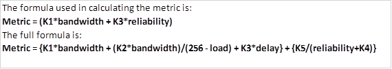
The K values are not used if they are 0.
NOTE: in as much as the above formulae are mentioned, CISCO recommends that you do not change them in the real world configuration of routers and as such, we will not discuss them any further. The metric will be discussed further in the CCNP level.
DUAL concepts
In the previous part, we mentioned that EIGRP uses the DUAL (Diffusion Update Algorithm) to calculate routes. In this section, we will learn how DUAL calculates the best paths and finds alternative or redundant loop free paths.
There are several terms we will discuss in this section. These terms are crucial to understanding EIGRP.
- Successor
- (FD) Feasible Distance
- (FS) Feasible Successor
- (RD) Reported Distance or (AD) Advertised Distance
- (FC) Feasibility Condition
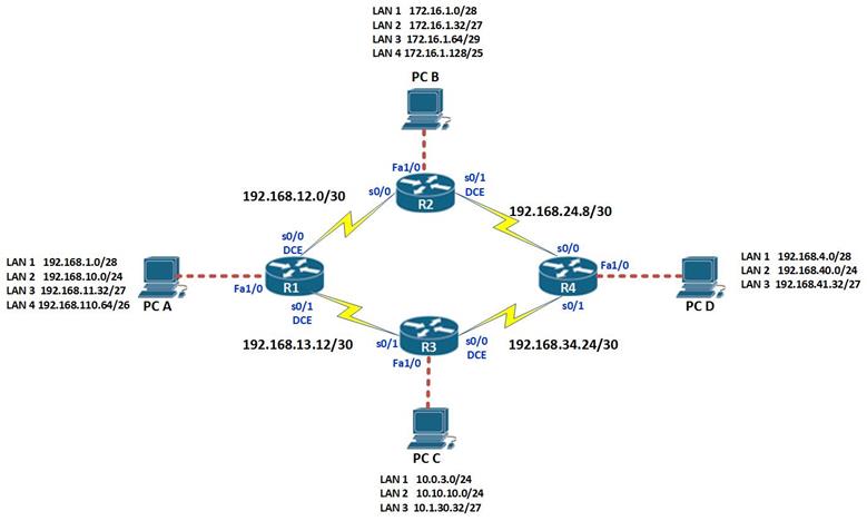
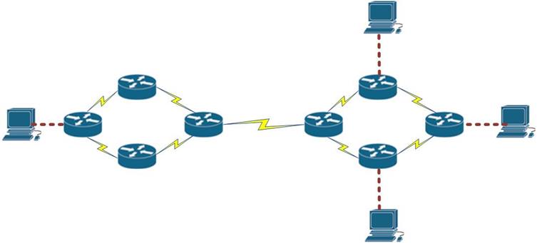
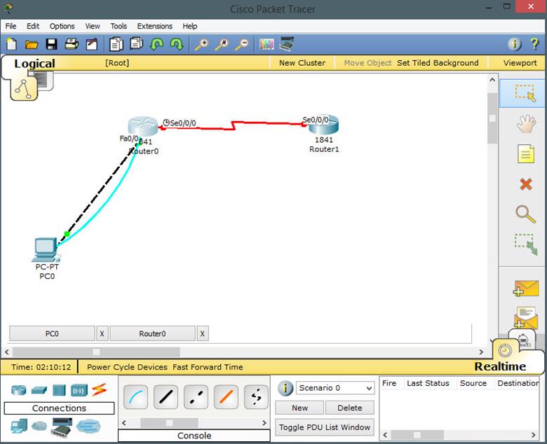
These terms are critical in understanding how EIGRP finds loop free paths. To understand these concepts better, we will use the topology shown below.
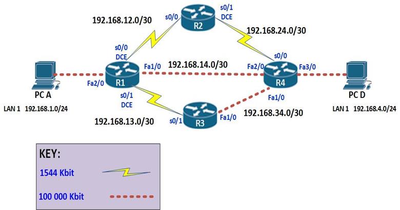
The topology above consists of 4 routers and 2 PCs. The connections are configured with the bandwidth shown in the Key which is the default for these types of links. EIGRP has been configured on all the four routers and the network is fully converged.
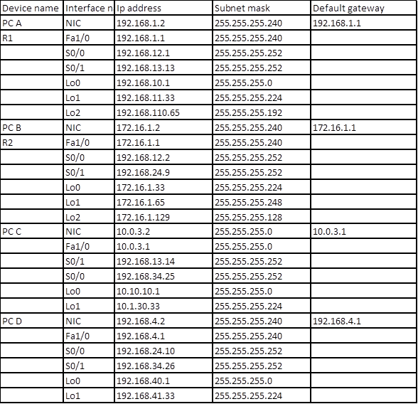
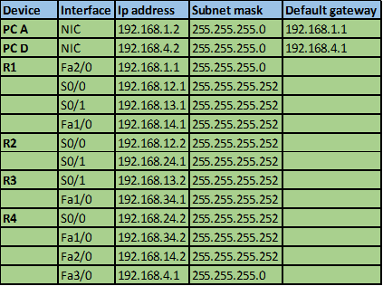
The ip addressing scheme is shown in the table below.
A successor in EIGRP is the neighbor router that is used to forward packets to a destination. This is a loop free path that has the lowest-cost or metric. By examining the ip route table in an EIGRP domain, the successor is the router that is shown with an IP address preceding the keyword “VIA”.
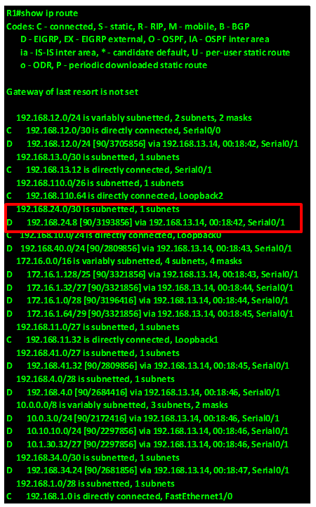
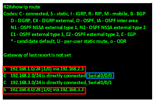
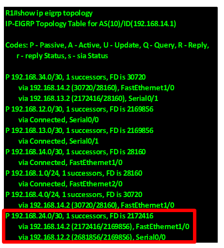
In our scenario, we can examine the routing table of R1 to determine the successor to network 192.168.4.0/24.
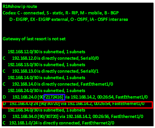
As you can see from the output above, highlighted in the RED box, the successor to the network 192.168.4.0/24 is via 192.168.14.2 which is the ip address of interface FastEthernet 2/0 on R4. Therefore the successor for this route is router R4.
Feasible Distance – is the metric that is used to reach a network. This is usually determined as the lowest cost loop free path by DUAL.
In the output above, the feasible distance to network 192.168.24.0/30 which is the link between R2 and R4 is shown in the blue box as 2172416.
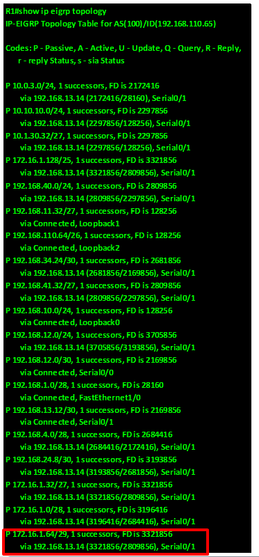
When a route goes down, EIGRP usually converges very quickly and uses a backup path if any, this is because the backup paths are usually calculated by DUAL algorithm and stored in the topology table.
The output of the “show ip eigrp topology” on R1 is shown below, and as you can see in the the highlighted section, the network 192.168.24.0 has 2 paths which are via 192.168.14.2 which is R4 and 192.168.12.2 which is on R2.
- . In the scenario shown below, the feasible distance to reach network 10.10.2.0/24 from R1 is equal to the distance between (R1 to R3) + distance from R3 to S1 which is equal to 110. The distance from (R1 to R4 ) + the distance from R4 to S1 is 220 therefore this is more costly.
REMEMBER: the lower the metric, the better the route

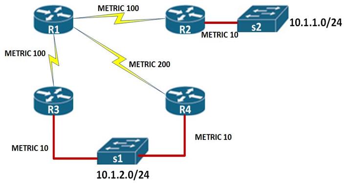
The advertised distance or the reported distance, is the metric to reach a network from the neighbor’s perspective.
In the scenario above, the reported distance to reach network 10.1.2.0/24 on R1, would be the distance from R3 to the switch, this is shown as 10 as indicated by the Red arrow above.
A feasible successor (FS) this is a neighbor who has satisfied the feasibility condition, and has a loop free redundant path for the successor.
The feasibility condition (FC) is the method that DUAL uses to determine whether a redundant path is viable. This condition usually states that the only way a path can qualify as a feasible successor is if, and only if, a neighbors Advertised Distance to a destination network, is less than the current successors feasible distance to that same network.
To better understand the feasibility condition, we use the diagram above with the explanation shown below.
In our scenario, above, the router R4 would be considered to be a feasible successor, if the distance from R4 to S1 is less than the distance from R1 to S1. i.e
The RD of network 10.1.2.0/24 through R4 is 10.
The FD of network 10.1.2.0/24 is 110
If 10 < 110, then this router satisfies the feasibility condition and can become the feasible successor.
In this topology, the feasibility condition has been met and therefore, the backup path to network 10.1.2.0/24 will be through R4.
NOTE: these concepts are very vital in understanding EIGRP and are often examined in the ICND 1, ICND 2 and CCNA composite exams.
These concepts will be explored further in CCNP level but they are a loop prevention measure in EIGRP.
Route summarization
EIGRP automatically summarizes at major network boundaries using the default auto-summary command. However, it is one of the most flexible routing protocols in that it allows for route summarization at any appropriate point in the network.
As we discussed earlier, automatic summarization can be disabled with the no auto-summary command in the router configuration mode for EIGRP. This command is shown below.
Router(config-router)#no auto-summary
Manual summarization
When doing manual summarization, we use a supernet route.
As discussed in the chapter on subnetting, a Supernet is a network address whose subnet mask is less than that of the classful mask in which it resides. If we have several subnets, we can summarize them to give a new address that will be advertised by the router.
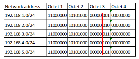
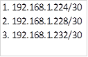
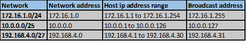
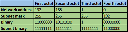
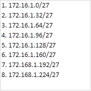
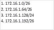
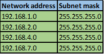
The table below shows five subnets that we need to summarize.
To summarize these addresses, we follow the following steps.
Step 1.
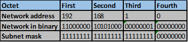
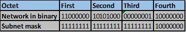
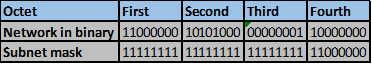
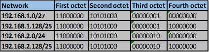
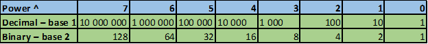
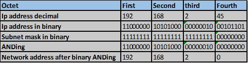
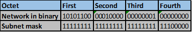
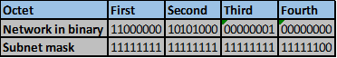
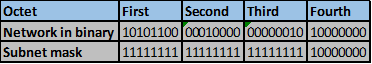
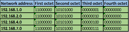
Convert the ip addresses to their binary equivalents as shown below.
Step 2.
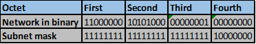
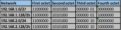
Consider the number of bits that match, when you find a column of bits that do not match, stop. You are at the summary boundary. In our scenario, the first 2 octets, and the first five bits in the third octet. Shown below by the red line.
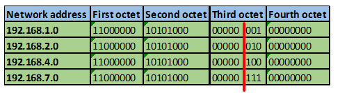
The total number of matching bits will be the new subnet mask, in our case this will be: the first two octets and the first five bits of the third octet.
REMEMBER: the subnet mask is comprised on ONLY “1s” on the network side, therefore in our case this will be:
255.255.248.0, this is the same as /21 in slash notation.
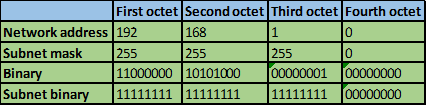
Now we need to determine the new network address.
Step 3. Determining the network address.
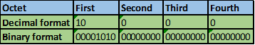
The network address is made up of the matching bits in the subnets. In our case, this will be:
192.168.0.0 since the matching bits in the third octet are only zeros. If we had “1s”, then the subnet mask would have been the addition of these values.
The supernet will be 192.168.0.0/21, this will be the summary address that will be advertised on a router which had the four subnets shown above.
In EIGRP, when advertising the summary address, we use the interface configuration mode. The summary address should be advertised out all the interfaces that participate in EIGRP. The command for configuring the summary address is as shown below:
Router(config-if)#ip summary-address eigrp <process-ID> <NETWORK_ADDRESS> <SUBNET_MASK>
The PROCESS_ID is the process ID that we used when configuring EIGRP.
The NETWORK_ADDRESS is the supernet that we derived from the manual summarization
The SUBNET_MASK is the new subnet mask for the supernet.
To understand manual summarization better, you should practice with different ip addresses.
Default route and route summarization configuration
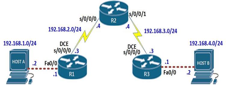
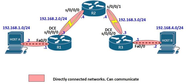
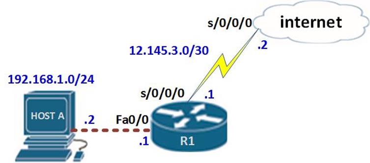
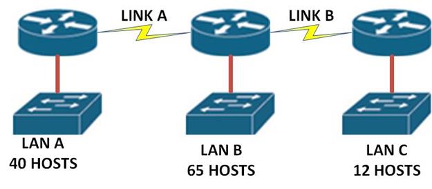
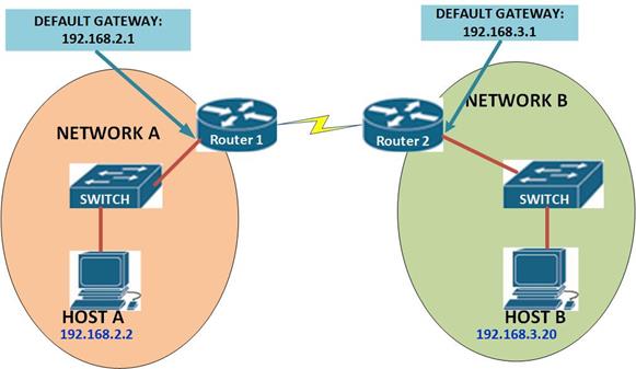
We may need to connect the enterprise’s network to other network such as the internet. Since we do not have control over these networks, we may need to configure a default route that will forward any unknown traffic to the internet. The scenario shown below will be the example we will use for this lab.
The topology consists of three routers; the interfaces in use are all shown. The two hosts PCs use the first useable ip address in their subnet, while the lan interfaces on the routers use the last useable ip address in their subnets as shown below.
Our task is to configure a default route and redistribute it in EIGRP so that R2 and R3 can access internet resources. Further, there are 5 loopback interfaces on R2 and R3, we should also configure summary addresses that will be advertised to R1.
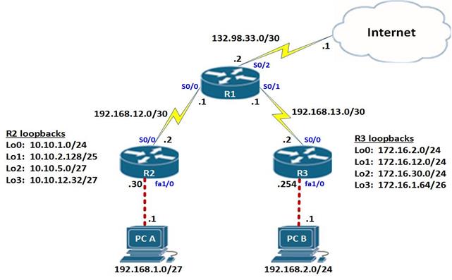
NOTE: to simulate a default route on the Internet, a network with the address 60.200.200.0/30 has been configured on the ISP.
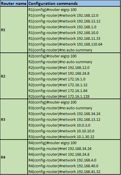
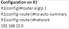
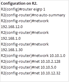
All the basic configurations including the ip addresses have been configured on the routers so we will just begin with the EIGRP configuration.
We will be using EIGRP AS 1 on all the routers.
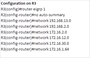
NOTE: when asked to configure EIGRP and there is a requirement to disable automatic summarization, this should be the first step. The configuration on the routers is shown below:
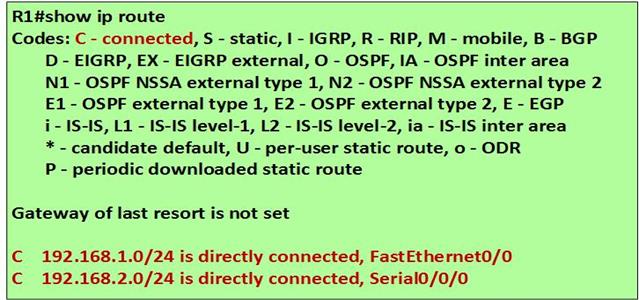
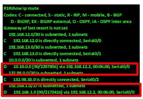
After this configuration, all routes should be propagated across the network except the default route. Now we need to examine the routing table of R1, to see how many routes it has.
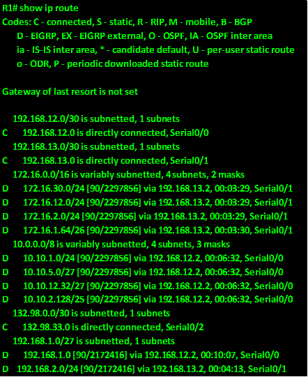
As you can see, we have 10 routes that we have learnt via EIGRP, we want to reduce this number and the way we can do this is by manual summarization of the loopback networks on R2 and R3.
Route summarization configuration
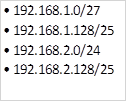
As mentioned earlier, the steps taken in supernetting of routes or route summarization are:
- Write out the networks that you want to summarize in binary.
- To find the subnet mask for summarization, start with the left-most bit.
- Work your way to the right, finding all the bits that match consecutively.
- When you find a column of bits that do not match, stop. You are at the summary boundary.
- count the number of left-most matching bits, this number becomes your subnet mask for the summarized route
- To find the network address for summarization, copy the matching 22 bits and add all 0 bits to the end to make 32 bits.
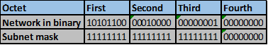
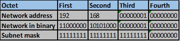
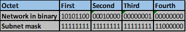
On R2, these steps are shown below.
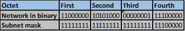
Step 1.
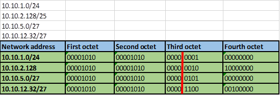
Step 2 -4.
The number of bits that match in this scenario are the first two octets and the first four bits in the third octet. This is indicated by the red line.
Step 5.
The number of matching bits are: 20 therefore the new subnet mask is 255.255.240.0
Step 6.
The new network address will be. 10.10.0.0/20
This is the summary address we will advertise out serial 0/0 on R2. The command used is shown below.
R2(config)#int s0/0
R2(config-if)#ip summary-address eigrp 1 10.10.0.0 255.255.240.0
Now we need to configure the same on R3 for its loopback networks.
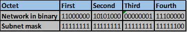
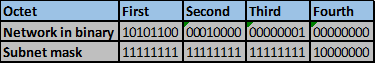
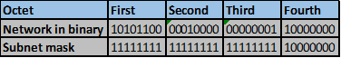
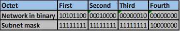
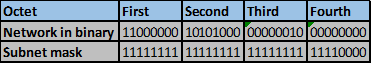
Step 1.
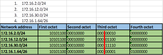
Step 2 -4.
The number of bits that match in this scenario are the first two octets and the first three bits in the third octet. This is indicated by the red line.
Step 5.
The number of matching bits are: 19 therefore the new subnet mask is 255.255.224.0
Step 6.
The new network address will be. 172.16.0.0/19
This is the summary address we will advertise out serial 0/0 on R3. The command used is shown below.
R3(config)#int s0/0
R3(config-if)#ip summary-address eigrp 1 172.16.0.0 255.255.224.0
After executing these two commands on R2 and R3, we need to look at the routing table of R1 to confirm whether we are getting the summary routes instead of individual routes as we saw earlier.
As you can see from the output above, R1 is now only receiving the summary routes from R2 and R3. These routes are highlighted in red.
Redistribute the Default route
To configure the default route, we follow the following steps.
Step 1. Configure a static default route on R1, this is done using the command:
R1(config)#ip route 0.0.0.0 0.0.0.0 s0/2
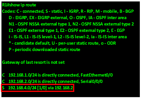
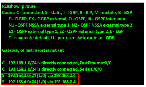
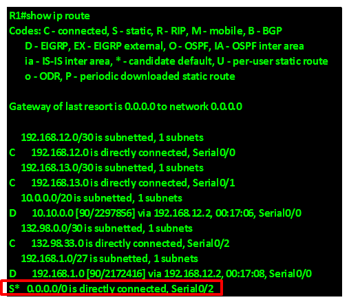
This will make any unknown traffic be forwarded out to the internet via serial 0/2 interface on R1. The routing table on R1 will now have this route as shown below in the red highlighted box.
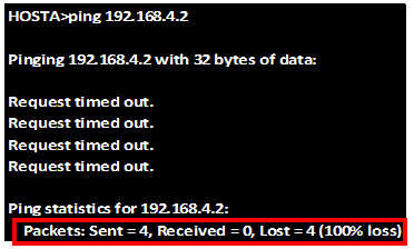
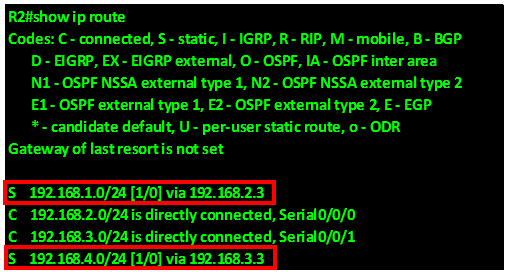
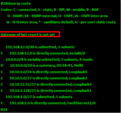
However, we also need R2 and R3 to forward unknown traffic to the internet and as you can see in the figure below, R2 does not have a default gateway in its routing table. This is also the case in R3. This means that any traffic destined to the internet from hosts on R2 and R3 will be dropped.
To solve this problem, we need to redistribute the static default route configured on R1 to R2 and R3.
In EIGRP, we need the redistribute command to enable the router configured with the static default update other routers in the EIGRP routing domain with the default route. This command when executed tells EIGRP to include the default route in its updates. When the routers in the EIGRP domain receive this route, they recognize it as the default route and add it to their routing tables.
The command on R1 is: R1(config-router)#redistribute static
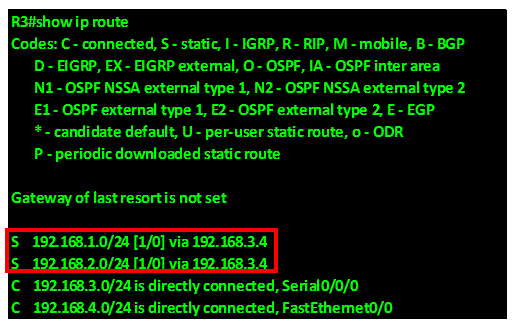
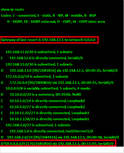
When this command is executed on R1, a new route should appear on both R2 and R3. The default route will now be redistributed on R2 and R3 as shown in R3’s routing table below.
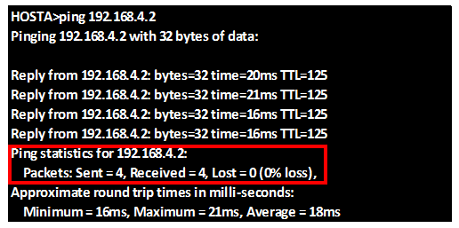
Now if we ping from PC_B to the network is in the internet we should be able to get replies, as shown in the output below. The ip address we will ping is 60.200.200.1.
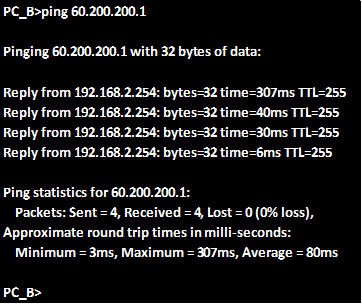
As you can see from above we are receiving replies from the ip address which is on the internet, which means that the default gateway has worked.
Passive interfaces
The final command that we will discuss in this chapter on EIGRP is the passive interface command. This command is used to limit the propagation of routing updates out of certain interfaces. In our networks, we need security, we do not need to send routing updates to areas where there are only end users such as our LANs. As such, this command is used to limit the EIGRP updates. When it is executed, this command will stop any routing updates out of a particular interface. In most cases, these are usually the LAN interfaces such as the FastEthernet links.
The command needed to configure passive interfaces in the EIGRP configuration mode is shown below.
Router(config-router)#passive-interface <interface_NAME><interface_ID>
Summary
In this chapter, on EIGRP, we have looked at the basics, and concepts behind the operation of EIGRP. We also discussed the dual concepts and did several lab configurations on EIGRP. In the CCNA exams, you will be presented with many questions on EIGRP and it is imperative that you understand this routing protocol well.
In the next chapter, we will look at link state routing protocols and especially OSPF, which is the last routing protocol we will discuss in this course.